
Labour Market Edition
March 2024

© Commonwealth of Australia 2024
ISSN: 2653-6196
This publication is available for your use under a Creative Commons Attribution 3.0 Australia licence,
with the exception of the Commonwealth Coat of Arms, the Treasury logo, photographs, images,
signatures and where otherwise stated. The full licence terms are available from
http://creativecommons.org/licenses/by/3.0/au/legalcode.
Use of Treasury material under a Creative Commons Attribution 3.0 Australia licence requires you to
attribute the work (but not in any way that suggests that the Treasury endorses you or your use of
the work).
Treasury material used ‘as supplied’.
Provided you have not modified or transformed Treasury material in any way including, for example,
by changing the Treasury text; calculating percentage changes; graphing or charting data; or deriving
new statistics from published Treasury statistics – then Treasury prefers the following attribution:
Source: The Australian Government the Treasury.
Derivative material
If you have modified or transformed Treasury material, or derived new material from those of the
Treasury in any way, then Treasury prefers the following attribution:
Based on The Australian Government the Treasury data.
Use of the Coat of Arms
The terms under which the Coat of Arms can be used are set out on the Department of the
Prime Minister and Cabinet website (see https://www.pmc.gov.au/honours-and-
symbols/commonwealth-coat-arms).
Other uses
Enquiries regarding this licence and any other use of this document are welcome at:
Manager
Media Unit
The Treasury
Langton Crescent
Parkes ACT 2600
Email: media@treasury.gov.au
In the spirit of reconciliation, the Treasury acknowledges the Traditional Custodians of country
throughout Australia and their connections to land, sea and community. We pay our respect to their
Elders past and present and extend that respect to all Aboriginal and Torres Strait Islander peoples.

Treasury Round Up | March 2024
Labour Market Edition | iii
Contents
Foreword .......................................................................................................................... iv
Labour market matching across skills and regions in Australia ........................................... 1
1 Introduction .................................................................................................................................................... 2
2 Matching efficiency in the Australian labour market ..................................................................................... 3
3 Skill level variation in labour market tightness and occupation movements ................................................. 7
4 Regional variations in labour market tightness and matching by skill level ................................................. 15
References ............................................................................................................................................................. 27
Exploring community resilience in Australia .................................................................... 29
1 Defining resilience ........................................................................................................................................ 30
2 Conceptualising the value of resilience ........................................................................................................ 31
3 Resilience frameworks .................................................................................................................................. 32
4 Measuring resilience .................................................................................................................................... 35
5 Conclusion .................................................................................................................................................... 40
Appendix ............................................................................................................................................................... 41
References ............................................................................................................................................................. 42
Employment behaviour of firms reliant on temporary migrants ....................................... 45
1 Temporary migrant workers ......................................................................................................................... 46
Incentives for secondary earners and income support recipients ..................................... 55
Address to the Policy Research Conference .......................................................................................................... 55
1 Introduction .................................................................................................................................................. 56
2 History of employment white papers ........................................................................................................... 57
3 The 2023 Employment White Paper ............................................................................................................ 58
4 The barriers framework ................................................................................................................................ 60
5 Secondary earners ........................................................................................................................................ 61
6 Income support recipients ........................................................................................................................... 64
7 Policy options ............................................................................................................................................... 66
8 Conclusion .................................................................................................................................................... 67

Treasury Round Up | March 2024
Foreword | iv
Foreword
Steven Kennedy
Broader indicators of labour market spare capacity are needed to measure progress towards
sustained and inclusive employment. Nearly 3 million people want to work, or to work more hours
than they do. The articles in this edition of the Round Up explore 4 aspects that are central to
addressing structural barriers in Australia’s labour market and meeting long-term labour market
objectives: geographical barriers, the net zero transformation, migration, and incentives.
As Australia faces changing skills needs across regions, improving job matching efficiency can support
greater economic output for a given level of labour supply and demand for workers. ‘Labour market
matching across skills and regions in Australia’ shows that matching efficiency has improved in recent
years, but that variations across labour market regions and skills can result in different labour market
outcomes across the country.
The net zero transformation is generating significant shifts across Australia’s economy and its regions.
The article ‘Exploring Community Resilience in Australia’ outlines the importance of resilience to
recover from and adapt to shocks. Not surprisingly, communities closer to major cities and regional
centres have higher levels of resilience compared to more remote communities.
The article ‘Employment behaviour of firms reliant on temporary migrants’ discusses how businesses
reliant on temporary migrants responded to Australia’s international border closure. The article finds
that businesses with higher temporary migrant workforces experienced greater job losses than
businesses less reliant on temporary migration. Businesses sought to find alternative labour sources
and to use labour more intensively. Observed increases in monthly average pay were likely driven by
increases in hours worked, and potentially due to increased hourly wages. Once borders reopened,
businesses responded by hiring more temporary migrants, with average pay of domestic workers
increasing by more than temporary migrants.
The final article is my address to the inaugural Treasury Policy Research Conference, which supported
the development of the 2023 Employment White Paper. The speech, ‘Incentives for secondary
earners and income support recipients’, finds that the tax-transfer system can shape decisions to
participate in the labour market, including decisions about how many hours to work. Secondary
earners and income support recipients may face reduced incentives to participate in the labour
market as fully as they may wish to. There are trade-offs between adequacy of government
payments, cost to taxpayers, and incentives to participate – all of which are important considerations
in the context of expanding labour market opportunities.

Treasury Round Up | March 2024
Labour market matching across skills and regions in Australia | 1
Labour market matching across skills and regions
in Australia
Will Mackey
1
Summary
This paper explores patterns of searching and matching in the Australian labour market. It first
estimates matching efficiency between 2004 and 2023 at the national level, showing 3 distinct
periods: a more efficient labour market leading up to the Global Financial Crisis; a decade-long
slump from 2010 with low matching efficiency and growing rates of long-term unemployed; and
a period of instability from 2020 when an unprecedentedly tight labour market was met with
strong job finding rates causing aggregate matching efficiency to rise throughout 2022.
Unemployed people were more likely to find work in 2022 than at any point since data began in
2004. This was true for short, long and very long-term unemployed people.
One source of mismatch – skill mismatch – is examined to show that higher skilled workers tend
to experience tighter labour markets and lower levels of within-skill mismatch compared to
lower-skilled groups. Between-skill employment mismatch means that higher skilled workers can
crowd out lower-skilled workers and job seekers.
The national labour market is then divided along regional and skill level lines to show
heterogenous conditions in 111 local labour markets. By controlling for some sources of
geographic and skill mismatch, this analysis demonstrates that mismatch remains within
region-skill labour market cells.
1 Thanks to Professor Jeff Borland, Stephanie Parsons, Josh Hickson, Nathan Deutscher, Omid Mousavi,
Phoebe Wilk, Oscar Lane, as well as other staff from Treasury and Jobs and Skills Australia, and
participants at the Australian Conference of Economists, for their thoughtful feedback and supporting
analysis for this paper. The views expressed are those of the authors and do not necessarily reflect those
of the Australian Treasury or the Australian Government.

Treasury Round Up | March 2024
Labour market matching across skills and regions in Australia | 2
1 Introduction
The Beveridge Curve is the relationship between job vacancies and job seekers in a labour market.
A tighter labour market indicates that there are more vacancies for each unemployed person, and a
looser labour market means there are more unemployed people for each vacancy. Chart 1.1 shows
Australia’s Beveridge Curve from the late 1970s to May 2023. There was high unemployment and low
vacancies in the late 1980s and early 1990s. The labour market tightened into the 2000s except for a
period of loosening at the onset of the Global Financial Crisis. The 2010s were relatively stable with
the vacancy rate of 1–2 per cent and unemployment rate between 4.5–6.5 per cent. With the
COVID-19 pandemic shock from 2020, unemployment grew temporarily before vacancies rose to the
highest level on record.
While these shifts reflect cyclical features of the labour market over time, how well job seekers and
jobs are ‘matched’ has an important role. Matching efficiency reflects the labour market’s ability to
match individuals to jobs, which can be limited by disconnects between the skills and location of
potential workers, and the requirements, renumeration, and location of available jobs. A more
efficient labour market will have lower levels of unemployment for the same level of labour demand.
Improving matching efficiency drives down the natural rate of unemployment and reduces skills
shortages in the economy.
Improving matching efficiency in the labour market means Australia can generate more economic
output for a given level of available workers and demand for labour. This paper first uses detailed
vacancy, job seeker and matching data to explore changes in labour market matching efficiency in
Australia between 2004 and 2023 for a range of job seeker groups. The paper then explores skill level
variation in labour market tightness and looks at occupation transitions within and between skill
groups. The final section adds a regional lens to illustrate the heterogeneity of local labour markets
that can coexist across Australia.
Chart 1.1 The Beveridge Curve
Source: Treasury analysis of ABS Job Vacancies and ABS Labour Force Survey. Seasonally adjusted figures.

Treasury Round Up | March 2024
Labour market matching across skills and regions in Australia | 3
2 Matching efficiency in the Australian labour market
Job vacancies and people looking for employment can coexist in the labour market. For example, a
skills mismatch can occur when a job seeker does not have the skills required for an available job, or
the job does not offer the required conditions or renumeration.
2
A geographic mismatch occurs when
the vacancy and job seeker are in different places and the job seeker is unable or unwilling to move.
Chart 2.1 Unemployment and
vacancy rates
Chart 2.2 Next-quarter job finding rate of
unemployed people
Source: ABS Labour Force Survey; ABS Job Vacancies.
Note: Original series. Vacancy rate interpolated
between 2008–09.
Source: ABS Labour Force Survey.
Note: Four quarter rolling average.
Matching efficiency describes the rate at which people seeking work are matched to vacant jobs in a
labour market.
3
Poor matching efficiency reflects disconnects between the preferences, skills and
location of potential workers, and the requirements, location, and renumeration of available jobs.
A more efficient labour market will have lower rates of unemployment for a given level of vacancies.
Improving matching efficiency in the labour market lowers the natural rate of unemployment,
reduces labour and skills shortages, and increases potential output.
While matching efficiency is not directly measured in the economy, it can be estimated from
measures of job vacancies, job seekers and job finders. Job vacancies are a measure of labour
demand. The ABS Job Vacancies series counts vacancies available for immediate filling, and the series
is correlated with near-term future employment growth. The vacancy rate was the highest on record
in 2022, almost double previous peaks (Chart 2.1).
2 A more detailed conceptualisation of labour market skills and skills shortages are outlined in
Richardson (2007).
3 The Beveridge Curve is the relationship between job vacancy and job seeker rates. Key Beveridge Curve
concepts are also explained in Figura and Waller (2022); Jobs and Skills Australia (chapter 5, 2021);
Anh and Crane (2020); Consolo and de Silva (2019); Borland (chapter 11, 2011).

Treasury Round Up | March 2024
Labour market matching across skills and regions in Australia | 4
Job seekers are all people who are seeking work. It is usually measured by the unemployment rate,
which is near a historic low (Chart 2.1). The ratio of vacancies to job seekers in a given period is a
measure of labour market tightness. A tighter labour market indicates there are more vacancies for
each unemployed person, and a looser labour market means there are more unemployed people for
each vacancy. Job finders are people who have a job in the current period and were seeking a job in
the previous period (Chart 2.2).
2.2 Unemployed matching efficiency
This paper measures matching efficiency over time using the job finding rate of unemployed people
relative to what would have been expected based on current labour market tightness (the ratio of
vacancies and unemployed). If job finding rates are unusually high (low), matching efficiency is
considered to be similarly high (low). This approach follows Consolo and de Silva (2019), which is
explored in more detail in Appendix A.
Matching efficiency of unemployed job seekers was high in the pre-GFC period between 2004 and
2009 (Chart 2.3). This period had decreasing unemployment, rising job vacancies, and high
job-finding rates for short-term unemployed. Job-finding rates were 1–3 percentage points higher
than expected for the level of labour market tightness. This period saw lower numbers of long-term
unemployed, who tend to have about half the job finding probability of short-term unemployed
(Chart 2.4).
Chart 2.3 Matching efficiency Chart 2.4 Job finding probability
Matching efficiency relative to long-run average Share unemployed who find work in the next month
Source: Treasury analysis, see Appendix A. Source: Treasury analysis of ABS Labour Force microdata.
Note: Four quarter average. Note: Four quarter average. Very short-term unemployed
is less than 4 weeks; short is 1–12 months;
long-term is >12 months.
Matching efficiency was low between 2010 and 2019. Labour market tightness had a partial rebound
after falling in 2009, but job finding rates remained below pre-GFC peaks across all unemployment
groups. Despite increasing labour market tightness from 2015, job-finding probabilities remained
relatively low. This was driven by lower job-finding rates of long-term unemployed, which made up
a larger share of the unemployed pool. Matching efficiency has been improving since 2019.

Treasury Round Up | March 2024
Labour market matching across skills and regions in Australia | 5
Matching efficiency started improving before the onset of the pandemic. Irregular labour market
conditions during 2020 caused measured matching efficiency to be unstable. A tight labour market in
the recovery from the pandemic has been matched by rising job-finding rates for unemployed
people. Unemployed people were more likely to find work in 2022 than at any point since data began
in 2004. This was true for short, long, and very long-term unemployed people.
2.3 Matching trends are clearer when more job seekers are
considered
People classified as unemployed are not the only people who seek and find work.
4
In addition to
unemployed job seekers, there are job seekers who are not in the labour force (NILF). These are
people who are not classified as unemployed but can be actively, passively, or not seeking
employment when previously surveyed. These NILF sub-groups are identified using ABS Labour Force
microdata (see Appendix A).
The first extension expands the scope of job seekers to include all non-working job seekers
(Chart 2.5).
Chart 2.5 Matching efficiency with
non-working job seekers
Matching efficiency relative to long-run average
Chart 2.6 Matching efficiency with all
job seekers
Matching efficiency relative to long-run average
Source: Treasury analysis of ABS Labour Force and ABS
Job Vacancies. See Appendix A.
Source: Treasury analysis of ABS Labour Force and ABS
Job Vacancies. See Appendix A.
When including all non-working job seekers this analysis finds better matching efficiency rates
between 2009–2013, driven by higher rates of NILF job seekers finding employment. This trend
reversed in subsequent years, pushing matching efficiency lower.
4 About twice as many people move from being outside the labour force to employment each period than
move from unemployed to employed. Capturing this group provides a fuller picture of matches and job
searchers in the Australian labour market.

Treasury Round Up | March 2024
Labour market matching across skills and regions in Australia | 6
Employed job seekers – workers who are looking for their next job – are also a large source of new
matches in the economy and can be identified using ABS Labour Force microdata. Adding employed
job seekers, the working and non-working matching efficiency rates were stronger before 2010, and
weaker between 2010 and 2021 (Chart 2.6). This follows trends in job-to-job transitions in the labour
force, which were high and rising until 2009. They then remained persistently low until recovering
from the end of 2021.
5
Trends in matching efficiency are relatively clear. Matching efficiency in the Australian labour market
started to improve in 2022 after a decade-long slump from 2008–2021. This means that unemployed
are finding work faster on average, after accounting for the time of year, vacancy rate and
unemployment rate, demonstrating that businesses are doing a better job at finding new employees
among the available pool of workers. Increased matching efficiency has been driven by all job seeker
groups – unemployed, NILF and employed. Two additional components of labour market matching –
skills and geography – will be explored in following sections.
5 Treasury analysis of ABS Labour Force microdata. See Deutscher (2019) for further discussions of
job-to-job transitions.

Treasury Round Up | March 2024
Labour market matching across skills and regions in Australia | 7
3 Skill level variation in labour market tightness and
occupation movements
Analysis of aggregate levels of labour demand (job vacancies) and labour supply (job seekers) is
useful for identifying cyclical trends at the national level. However, the Australian labour market is not
a single, homogenous market. For example, a nurse vacancy in Perth is unlikely to be filled by an
unemployed construction labourer in Cairns, and high unemployment rates of construction labourers
in Cairns are unlikely to fall by hiring more nurses in Perth. This section explores skill level and
occupational labour market matching.
3.1 Exploring skilled labour markets within Australia
The identification of specific labour markets can help us understand sources of mismatched supply
and demand across skill and geographic lines and inform labour market policy decisions. To explore
the labour markets that exist beneath the aggregate requires measuring job vacancies and job
seekers along common dimensions, when:
• Vacancies only have characteristics associated with a particular job, such as an occupation, an
industry, a location and an advertised wage, and
• Job seekers have characteristics only associated with a person, such as: age, sex, a level and field
of education, a location of residence, and – for those who have been recently employed – an
occupation and industry of their previous job.
This analysis uses a job vacancy’s occupation and individual job seeker education level and previous
occupation to explore labour supply, demand, and matching levels by skill levels.
6
Three skill
groupings are used – low, middle and high – which correspond to occupation skill and education
levels. The exact methodology is outlined in Appendix B.
This classification allows for people working in high (or middle) skill occupations to be classified as
high (or middle) skill workers, regardless of their education, to reflect skills developed through
workforce experience. The inclusion of education allows for people without a current or previous
occupation, such as new entrants to the workforce or those coming back from extended periods of
leave or long-term unemployment, to be classified by their education level. This approach means that
every person in the labour force can be assigned a skill level.
7
However, due to data limitations before
August 2015, this analysis is restricted to 2016 onwards.
Applying these skill level groupings to job vacancies and unemployed people in Australia shows
distinct characteristics of high, middle and low-skill labour markets compared to the aggregate.
6 This definition of ‘skill’ is common in the literature and is used by the ABS to form its occupational skill
level framework: ABS (2022). However, this definition of skill does not include or measure the full range of
skills and abilities required by occupations, or for specific jobs within occupations, or those performed by
individuals within their job. Jobs and Skills Australia (2023) provides detailed descriptions of specific skills
that are required for individual occupations in its Australian Skills Classification. See Richardson (2007) for
a detailed discussion of labour market skills.
7 Alternative approaches that rely solely on a person’s previous occupation to determine their skill level are
unable to classify a significant share of the job seeker pool, particularly long-term unemployed and new
entrants to the workforce.

Treasury Round Up | March 2024
Labour market matching across skills and regions in Australia | 8
Chart 3.1 shows unemployment rates and vacancy rates for each labour market. In the aggregate
labour market (Panel A), as explored in Section 1, the vacancy rate rose slightly between 2016 and
2019, before dipping in 2020 with the onset of COVID-19. From mid-2020, vacancies rebounded
before surpassing previous levels and now sit at about 3.5 per cent of labour demand (employment
plus vacancies). The unemployment rate has moved broadly inversely to the vacancy rate.
The high-skill labour market (Panel B) tends to be tighter than the aggregate. Demand for high-skill
occupations followed a broadly similar path to the aggregate trend, with a slightly lower vacancy rate
(less than 2 per cent) before increasing to 2.3 per cent at the beginning of 2023. The high-skill group
tends to have low unemployment rates, from about 3.5 per cent between 2016 and 2019 to less than
2 per cent in 2023. At the beginning of 2023 there were more vacancies for high-skill jobs than there
were job seekers with high-skill occupations. However, low unemployment rates may overstate the
level of matching efficiency in the high-skill labour market, as many people are employed in lower-
skilled occupations (explored in the next section).
The middle-skill labour market (Panel C) is persistently looser than the high-skill group, with higher
unemployment and marginally lower labour demand. However, the middle-skill labour market has
tightened significantly over the past 2 years, in line with the aggregate labour market.
The low-skill labour market (Panel D) has higher rates of unemployment and higher rates of
vacancies. The low-skill labour market has tightened significantly since mid-2020, with declining
unemployment rates and rising vacancy rates. But within-skill level mismatch remains high, with
about 7 per cent of the labour force unable to be matched to available jobs. In addition, low-skill job
seekers also compete with some higher skilled job seekers, as explored in the next section.
Chart 3.1 Unemployment and vacancy rates by skill group
Source: Treasury analysis of ABS Longitudinal Labour Force Survey, ABS Job Vacancies, JSA Internet Vacancy Index.
See Appendix B.

Treasury Round Up | March 2024
Labour market matching across skills and regions in Australia | 9
3.2 Skill level mismatch of workers can ‘crowd out’ lower-skill
workers
Some degree of skill level mismatch will always exist in the labour force. Over education – where a
worker is in an occupation that does not require their level of education – has increased alongside
rising educational attainment. Sometimes people optimally choose a job that is different to their level
of education and training, reflecting the personal preferences of workers. Other times it is
undesirable, caused by temporary and structural factors that can have flow-on effects to others in the
labour force.
Skill level misallocation may hint at some labour market challenges
Labour market tightness in the high-skill market sits alongside apparent between-skill mismatch.
The mismatch between a worker’s education level and their occupation level is significant. Between
2016 and 2023, about 30 per cent of high-skill workers were employed in occupations classified as
middle and low-skill. This is consistent with other research on over education in the Australian labour
market.
8
These occupations were often lower-skilled health and clerical or administrative roles
(Chart 3.2). Over 40 per cent of middle-skill workers were employed in low-skill occupations,
particularly as machinery operators and labourers.
Skill level mismatch can be the consequence of a more educated workforce. There has been
significant growth in bachelor and postgraduate degree attainment over the past 40 years. About
40 per cent of 25 to 34-year-olds had a bachelor’s degree or above in 2020 (up from 10 per cent in
1980).
9
Over education can be temporary or reflect other compensating factors, such as location or
flexibility or lower pressure jobs.
Skills depreciation can also drive apparent skill level mismatch. The skills demanded within some
occupations can change quickly.
10
Workers who spend time away from the workforce or from a
particular occupation can find themselves without the skills now required for their job, despite having
the required level of education.
Job skill misclassification can occur when a particular job within an occupation requires more
education than is typically required for that occupation. For example, the education and training
requirements for a Hospitality Manager can vary according to the size and complexity of the
organisation.
Geographic mismatch, where appropriately skilled jobs are not available in the region, can also lead
job seekers to take up lower-skilled work. This type of mismatch is explored in Section 4.
8 Heath (Graph 11, 2020). While education and occupation skill level definitions of skills mismatch are
presented in this paper, Treasury analysis of HILDA data also finds that about 25 per cent of people with
post-secondary qualifications self-report that their skills are not well utilised in their current job.
9 Rates of vocational attainment have remained flat over this period at about 35 per cent. Norton,
Cherastidtham and Mackey (Figure 1.1, 2019).
10 Deming and Noray (2020) demonstrate this effect in the United States, showing that skill obsolescence
lowers the income returns to work experience in faster-changing occupations.

Treasury Round Up | March 2024
Labour market matching across skills and regions in Australia | 10
Chart 3.2 Share of employees by skill
Source: Treasury analysis of ABS Longitudinal Labour Force Survey.
Note: Occupation is ANZSCO submajor, and skill level as defined in Appendix B. Data are pooled across 2016–2023.

Treasury Round Up | March 2024
Labour market matching across skills and regions in Australia | 11
Many people (re)enter the labour market in lower-skilled jobs
Skill level mismatch also means that low-skill job seekers have to compete with high and middle-skill
job seekers for the same roles. Chart 3.3 on the following page shows the next quarter destination
occupations for unemployed people without prior occupation information. This group contains young
job seekers, about half of whom are entering the workforce for the first time. It also includes those
who have been without an occupation for an extended period – such as those coming from periods
of leave or long-term unemployment.
Low-skill workforce entrants are most likely to find employment in Sales Assistant (20 per cent) and
Sales Support (6 per cent) roles; in Hospitality (12 per cent) and Food Preparation (10 per cent) roles;
and as Cleaners (6 per cent), Drivers (5 per cent) and Other Labourers (5 per cent).
Middle-skill workforce entrants have access to a broader range of jobs, especially as Carer and Aides
(13 per cent) and trades, such as Construction (5 per cent) and Automotive Engineers (5 per cent).
However, middle-skilled workforce entrants also find work in lower-skilled occupations. For example,
6 per cent enter Sales Assistant roles, an occupation that typically does not require a qualification.
High-skill workforce entrants are more concentrated among education, health, and business
professional roles. About a third of high-skill workforce entrants find work in lower-skilled
occupations. These patterns follow the over education patterns (Chart 2.2), with lower-skilled health
and administrative jobs being common.
Workers switch jobs across skill levels but within clusters
As with new entrants to the labour market, workers who switch jobs compete with unemployed
people for vacancies. Much of this job switching is within the same occupation. There is some
movement from one skill level to another when people switch occupations. Workers and job seekers
have preferences, foundational skills, and specialised skills required for occupations that shape the
roles they look for in the labour market.
Preferences for the type of work a person wants to pursue develop over time and are affected by
factors including socio-economic status, occupational segregation (such as by sex), and
macroeconomic conditions during childhood.
11
Foundational skills developed through education and workplace experience – such as
communication, teamwork and problem solving – are common across a range of occupations and can
allow workers to switch occupations.
12
11 For example, these preferences are affected by: socio-economic status during childhood, Gore (2015); by
macroeconomic conditions when growing up, Cotofan, Cassar, Dur & Meier (2023); and by gender
stereotypes and highly segregated occupations, Women’s Budget Statement (pp 28–30, 2023).
12 The importance of these foundational skills in a changing labour market is outlined by the National Skills
Commission (pp 146–151, 2021). An examination of the growing importance of – and returns to – social
skills in the labour market is explored in Deming (2017).

Treasury Round Up | March 2024
Labour market matching across skills and regions in Australia | 12
Chart 3.3 Unemployment to employment transition rates for people with no prior
occupation
Source: Treasury analysis of ABS Longitudinal Labour Force Survey.
Note: Occupation is ANZSCO Submajor, and skill level group is defined in Appendix A. Data are pooled across 2016 to
2023.

Treasury Round Up | March 2024
Labour market matching across skills and regions in Australia | 13
Specialised skills can be specific to a particular job, occupation or industry. These skills tend to be
developed over long periods – through education, training and work experience – and tend to be less
transferable than foundational skills. For example, a school teacher is unlikely to have the skills to
take up a job as a registered nurse, despite the same education level and similar foundational skill
requirements. However, some occupations overlap in specialised skills.
13
While numerical clerks,
business professionals and chief executives are distinctly different occupations, they all require
numerical skills.
Preferences, foundational and specialised skills interact to form clusters of occupational transitions in
the labour market. These clusters can be explored using a transition matrix of job changes. Case
studies are presented in Chart 3.4 to illustrate the patterns of within/between occupation transitions.
• Of business professionals who begin with a new employer, about a third move into specialised
management roles, while 15 per cent remain as business professionals. There is some transition
within the professional environment, particularly into design IT and education. A smaller share
move to lower-skilled occupations that require skills developed in business, such as numerical
clerks and office administrators.
• Of health professionals who begin with a new employer, almost 40 per cent stay within the health
professional occupation. For those who move, the most common destination is to specialist
management. There is also some down-skilling, with moves most likely to health and welfare
support, and carer occupations.
• Automotive engineers are the most likely to stay within their occupation of these case studies,
with about half remaining as automotive engineers after a move to a new employer.
• Carers and aides also have relatively high within-occupation retainment. New occupations tend to
be to health and support workers, or to higher skilled occupations as education or health
professionals.
• Construction and mining labourers tend to move to other manual occupations, with about
two-thirds moving to similar labourer jobs, such as factory or forestry workers, or to machine
operators and driver occupations. About 20 per cent move to trades occupations that tend to
require qualifications, particularly construction trades.
Between-skill mismatch means that significant shares of high- and middle-skill workers are in
occupations that may not make best use of their skills. While most entrants to the workforce find
work aligned with their skill levels, many high- and middle-skilled job seekers find work in lower-
skilled occupations. Geographic mismatch – job opportunities and job seekers being in different
regions – can play a significant role in the efficient working of the labour market. This is explored in
the next section.
13 The similarity of occupations by specialised skills are explored in the Jobs and Skills Australia Australian
Skills Classification (2023).

Treasury Round Up | March 2024
Labour market matching across skills and regions in Australia | 14
Chart 3.4 Select occupation-to-occupation transitions
Destination occupations (rows) as a share of newly employed original occupations
Source: Treasury analysis of ABS Longitudinal Labour Force Survey, ABS Job Vacancies, JSA Internet Vacancy Index.

Treasury Round Up | March 2024
Labour market matching across skills and regions in Australia | 15
4 Regional variations in labour market tightness and
matching by skill level
4.1 Exploring labour markets by skill and region
Australia is not a single homogenous labour market. Many factors drive local labour demand and
supply within regions. This means labour market conditions can vary significantly. Cyclical and
structural forces can have different effects on labour demand in regions based on their industrial
composition. Labour supply can respond differently based on its skills mix and demography.
Australia is a large country and geographic mismatch – job opportunities and job seekers being in
different regions – can play a significant role in the efficient working of the labour market. As the
majority of work is done in person, strong demand for labour in one corner of the country is unlikely
to materially reduce unemployment in another corner. Geographic mobility can provide some
solutions to this mismatch. However, this is not a viable option for all jobs or for all job seekers.
The analysis in this section examines the supply of and demand for skilled labour in each region in
Australia. It identifies overall regional trends in tightness and mismatch by skill level, before
examining a series of regional labour markets with distinctly different outcomes.
Geographic mobility is a partial solution to geographic mismatch
Geographic mismatch occurs when there are job seekers and appropriate job vacancies in different
regional labour markets. Geographic mobility – workers coming to jobs, jobs coming to workers, or a
mix of the two – is one tool to reduce geographic mismatch.
• Workers permanently moving to jobs: young people are more likely to move.
14
There is also a
higher propensity for geographic mobility among renters, unemployed and underemployed
people.
15
However, people are most likely to move within the same labour market because of
housing or family reasons rather than work. People who are more established in an area – such as
those with children and those who own their own home – are less likely to move. Long-term
unemployed also face additional challenges in moving long distances in search of work.
16
• Workers moving to jobs via long distance commuting: for employers and employees who cannot
or will not permanently move location, fly-in fly-out (FIFO) and drive-in drive-out (DIDO) provides
an alternative pathway for managing geographical mismatch. This approach has been a defining
characteristic of Australia’s mining booms with significant population shares of mining regions
appearing to be FIFO workers.
17
Long distance commuting is also playing a role in hybrid
arrangements with remote work.
14 Administrative data published by the ABS (2023).
15 Whelan and Parkinson (2017); Productivity Commission (Chapter 7, 2014).
16 Productivity Commission (Chapter 7, 2014). The Productivity Commission also noted that ‘longer distance
moves for the purpose of finding work are likely to be challenging for many long-term unemployed people
due to lower levels of education and skills, poorer health, less access to affordable transport and greater
reliance on family networks for support’ (p 147).
17 D’Arcy, Gustafsson, Lewis and Wiltshire (2012).

Treasury Round Up | March 2024
Labour market matching across skills and regions in Australia | 16
• Jobs moving to workers via remote work: remote work is an option in some jobs. This allows
workers and jobs in different regions to be matched.
The region-skill Beveridge Curve
This analysis splits the labour market into 37 regions and 3 skill groups (used in Section 3) to explore
111 region-skill labour markets in Australia between 2016 and 2022 (see Appendix D).
These regions are used to allow the use of JSA Internet Vacancy Index data by region and can provide
an overview of regional labour market characteristics. However, some regions span particularly large
areas, meaning that some geographic mismatch remains even when looking at specific regions.
All quarterly observations for the region-skill labour market cells are presented in Chart 4.1. It shows
that the high-skill group has persistently lower rates of unemployment for a given vacancy level than
middle or low-skill groups. Across regions, low-skill groups tend to have higher unemployment and
vacancy rates.
Low and middle-skill groups tend to be below the ‘ ’ line (where vacancies equal
unemployment). However, there are some outliers that sit above that line, with greater vacancies
than unemployed within or across skill groups. These areas tend to be in smaller capital cities.
Chart 4.1 Beveridge curve by skill and geography, 2016–2022
Each point represents a quarterly observation of a skill group in a labour region. Log scales.
Source: Treasury analysis of ABS Longitudinal Labour Force Survey, ABS Job Vacancies, JSA Internet Vacancy Index.

Treasury Round Up | March 2024
Labour market matching across skills and regions in Australia | 17
4.2 Different labour market conditions across regions
The methodology developed across this, and the previous sections, allows us to measure labour
market conditions over time for individual labour markets (within skills and within regions).
The analysis shows that a broad range of labour market conditions exist within Australia at any point.
Case studies are presented in the figures below to illustrate these structural and temporary
differences. The following figures show unemployment rates and vacancy rates for each region-skill
labour market.
Sydney: Similar trends to national average
The Sydney labour market tends to have higher demand and similar unemployment levels to the
national average. The overall vacancy rate (Panel A) was relatively flat between 2016 and 2019,
before dropping quickly in 2020 and rebounding to surpass previous levels (Chart 4.2). The
unemployment rate has moved broadly inversely to the vacancy rate.
The high-skill labour market (Panel B) tends to be tighter than the middle and low-skill labour
markets. The middle-skill labour market (Panel C) is persistently looser than the high-skill group, with
higher unemployment and lower labour demand. However, the middle-skill Sydney labour market has
tightened significantly over the past 2 years, in line with the national labour market.
The low-skill labour market (Panel D) has higher rates of unemployment and higher rates of
vacancies. Low-skill labour demand in Sydney grew rapidly since mid-2020. Unemployment rates
followed, starting to decline from early 2021 and by 2023 were below pre-pandemic levels and rising
vacancy rates. But within-skill level mismatch remains high, with about 8 per cent of the labour force
unable to be matched to available jobs.
Chart 4.2 Sydney unemployment and vacancy shares by skill group
Source: Treasury analysis of ABS Longitudinal Labour Force Survey, ABS Job Vacancies, JSA Internet Vacancy Index.

Treasury Round Up | March 2024
Labour market matching across skills and regions in Australia | 18
Darwin: Persistent within-skill labour shortages
Darwin has had a tighter labour market than the national average, with about the same number of
unemployed job seekers and job vacancies between 2016 and 2019 (Chart 4.3).
During this time, there was an excess of high-skill labour demand and an excess of low-skill labour
supply. From 2022, the Darwin labour market has had a significant excess of labour demand.
This trend has been seen across all skill levels.
While unemployment rates in Darwin are similar to national levels, vacancy rates are elevated across
all skill groups. This indicates that more jobs and job seekers coexist in the same region within the
same skill level, but face higher levels of within-skill mismatch. Darwin has had a persistent shortage
of workers in across the 3 skill groups since 2021.
Chart 4.3 Darwin unemployment and vacancy shares by skill group
Source: Treasury analysis of ABS Longitudinal Labour Force Survey, ABS Job Vacancies, JSA Internet Vacancy Index.

Treasury Round Up | March 2024
Labour market matching across skills and regions in Australia | 19
Toowoomba and South West Queensland: Persistent loose labour market
Toowoomba and South West Queensland (Chart 4.4) had a persistently loose labour market between
2016–2023.
While unemployment tends to be lower for high-skilled groups, unemployment remains higher across
all skill groups than the national average. People in the low-skill labour market have experienced
particularly high rates of unemployment.
This is at least in part reflected in low levels of labour demand, with vacancies below national levels
across skill groups, especially for low-skill occupations.
Chart 4.4 Toowoomba and South West Qld unemployment and vacancy shares by skill
Source: Treasury analysis of ABS Longitudinal Labour Force Survey, ABS Job Vacancies, JSA Internet Vacancy Index.

Treasury Round Up | March 2024
Labour market matching across skills and regions in Australia | 20
Far North Queensland: Long-run tightening labour market
Far North Queensland (Chart 4.5) has an increasingly tight labour market with average levels of
matching efficiency. Unemployment decreased from 2016–2022 across skill groups. Overall, the
unemployment rate has declined from about double the national rate to the national rate in 6 years.
The unemployment rates of low-skill workers were above 18 per cent in 2016 and have progressively
decreased to below 8 per cent by the end of 2022. The reduction in unemployment has been allowed
by rising demand for labour over this period across all skill levels.
Chart 4.5 Far North Queensland unemployment and vacancy shares by skill group
Source: Treasury analysis of ABS Longitudinal Labour Force Survey, ABS Job Vacancies, JSA Internet Vacancy Index.
4.3 Summary
Australia is made up of heterogenous labour markets, each of which can have different levels of
mismatch and labour market tightness. Some regions experience acute labour or skills shortages at
the same time others have persistently high rates of unemployment. However, much of Australia’s
labour market mismatch is within region and skill groups. In many regions, including in most major
cities, labour supply and demand is currently close to parity. Low-skill regional labour markets in
particular demonstrate high levels of unemployment and high levels of job vacancies, suggesting
within-region, within-skill group matching efficiency needs to improve to further reduce
unemployment.

Treasury Round Up | March 2024
Labour market matching across skills and regions in Australia | 21
Appendices
Appendix A Modelling matching efficiency
This paper estimates aggregate matching efficiency following Consolo and de Silva (section 3, 2019).
18
This approach specifies the matching function as a constant returns to scale Cobb-Douglas function of
the vacancy rate and the unemployment rate.
Following their approach, the aggregate matching function is estimated by looking at quarterly job
finding probabilities and labour market tightness (the vacancy-unemployment ratio), with matching
efficiency defined as the time-varying residual from estimating a reduced form matching function.
19
An adjusted version of the Consolo and de Silva (equation 1, 2019) model is:
20
and
(1)
where matching probability
is the share of job searchers the previous period
who found a
job in the current period,
. Labour market tightness,
, is the ratio of job vacancies
and job
searchers,
.
is a control for quarter to account for regular seasonal effects. The residuals,
, can
be interpreted as a measure of matching efficiency in the current period. In what follows, we describe
our implementation of this approach in the Australian setting.
For all models, the period is quarterly and the measure of vacancies in the economy is ABS Job
Vacancies.
21
Different measures of job searchers (and, therefore, matching probability) are explored
in 3 models:
A. Unemployment model: the unemployment model follows a standard Beveridge Curve
framework – and that used in Consolo and de Silva (2019) – by defining job searchers as
unemployed people,
. Unemployment data is sourced from the Labour Force Survey.
22
18 For more detail about how this approach fits into the Beveridge Curve framework, see Consolo and
de Silva (Box 2, 2019); Petrongolo and Pissarides (2001); and Figura and Waller (2022).
19 The authors show that in the European context from 2000, the reduced form matching function approach
reveals similar matching efficiency estimates to an alternative measure derived by estimating the elasticity
between vacancies and unemployment: Consolo and de Silva (equation 2 and chart 5, 2019).
20 A polynomial term
is added to account for potential non-linearity in the relationship between labour
market tightness and job finding probability. The findings in this paper are robust to the removal of this term.
21 ABS Job Vacancies (Australia: Table 1; and states: Table 2). Job vacancy data was not collected between
August 2008 and August 2009 and is linearly interpolated for analysis conducted in this paper.
22 ABS LFS, Table 1. Original series are used. State-based analysis also uses this model, with data coming from
Table 12. Job finding probabilities of unemployed people is sourced from ABS LFS Flows into and out of
employment (GM1).

Treasury Round Up | March 2024
Labour market matching across skills and regions in Australia | 22
B. Non-workers model: expands the definition of job searchers to include NILF job seekers,
. Three groups are considered to be possibly searching for employment within the
NILF cohort: those actively searching for work, those passively searching for work, and those not
searching for work.
23
ABS Longitudinal Labour Force microdata is used to determine how many of
each group enter employment in each period. The number of job searchers in each group is
defined as the number of job finders divided by the hiring rate of the actively looking group.
24
C. Workers and non-workers model: adds employed job searchers to the non-workers model,
including all job searchers in the labour market:
. ABS Longitudinal Labour
Force microdata is used to count the number of new hires from the employed pool, measured
using the share of previously employed workers who have been in their current job for less than
3 months. The share of job searchers who are seeking work at any point is assumed to be fixed at
10 per cent.
23 Treasury research by Parsons and Hickson (2022) [unpublished] shows the ‘not looking for work’ NILF
group is the largest group, accounting for just under half of the whole NILF group. Those who are retired
or permanent unable to work, the second largest NILF group, are excluded. This group has very low levels
of job finding.
24 The intuition is that a NILF person will move from ‘not looking’ or ‘passively looking’ to ‘actively looking’
before finding a job, even if they are only ever measured as being ‘not looking’ in one period and
‘employed’ in the next.

Treasury Round Up | March 2024
Labour market matching across skills and regions in Australia | 23
Appendix B Defining skill level groups
This analysis defines skill levels to match vacancies (which have occupations) and unemployed people
(who have education levels and, often, a previous occupation).
Method
In this analysis, skill level is defined as one of 3 exclusive and exhaustive groups:
• High skill: Bachelor’s degree or above required, ABS skill level 1
• Middle skill: Cert III/IV or diploma required, ABS skill level 2 or 3
• Low skill: High school or Cert I/II required, ABS skill level 4 or 5.
A job vacancy’s skill group is defined by the ABS skill level of its ANZSCO occupation. A person’s skill
group is defined by their highest level of education or the skill level of their current or previous job.
• Education level is important to define the skill levels of people without information on their
previous occupation. This group is largely made up of young job seekers, about half of whom are
entering the workforce for the first time. It is also comprised of those who have been without an
occupation for an extended period, such as those coming from periods of leave or long-term
unemployment. Education information has only been collected for each rotation group in the ABS
Longitudinal Labour Force since August 2015.
• Note that as people are classified by the highest education and occupation skill level, this style of
analysis cannot identify ‘under skilled’ workers. By definition a worker without a bachelor’s degree
working in a high-skill occupation that would usually require a bachelor’s degree is classified as
high skill.
Data
• Skill level vacancy shares are taken from the JSA Internet Vacancy Index (by ABS skill level and
state), with state shares scaled to state job vacancy levels from ABS Job Vacancies.
• Skill level employment and unemployment shares are generated from ABS Longitudinal Labour
Force microdata using an individual’s highest level of education and ABS skill level of their current
or previous occupation. ABS skill levels and education levels are then assigned a high, middle or
low-skill grouping according to the method described above.
• Skill level shares are scaled to publicly available employment and unemployment counts from the
ABS Labour Force Survey (original series, not seasonally adjusted).

Treasury Round Up | March 2024
Labour market matching across skills and regions in Australia | 24
Appendix C Occupation transition matrices
ABS Longitudinal Labour Force microdata is used to explore changes in ANZSCO sub-major occupation
for individuals from one quarter to the next. These labour force transition matrices allow us to see
where all people, including unemployed people and those without a previous occupation, tend to
gain employment by occupation when commencing a new job. All transitions observed between 2016
and 2022 are pooled to generate the matrix to avoid sample size issues.
Chart C.1 on the following page shows the full transition matrix.

Treasury Round Up | January 2024
Labour market matching across skills and regions in Australia | 25
Chart C.1: Occupation transitions for people commencing new jobs
Source: Treasury analysis of ABS Longitudinal Labour Force Survey.
Note: Pooled quarterly transitions between 2016–2022.

Treasury Round Up | January 2024
Labour market matching across skills and regions in Australia | 26
Appendix D Defining region-skill groups
This analysis defines regions and skill levels to match vacancies (which have locations and
occupations) and unemployed people (who have locations, education levels and previous
occupations).
This analysis splits labour market into 37 regions with 3 skill groups (111 cells) to explore varied
conditions. Regions are defined by JSA Internet Vacancy Index (IVI) Regions. Labour force data is
sourced from the ABS Longitudinal Labour Force microdata at Statistical Area 4 (SA4) level before
being corresponded to IVI regions. JSA provides a correspondence tables of SA4 regions to IVI
regions.
These regions are shown in Chart D.1.
Chart D.1: Internet Vacancy Index regions
Source: Jobs and Skills Australia (2023).

Treasury Round Up | January 2024
Labour market matching across skills and regions in Australia | 27
References
Australian Bureau of Statistics. (2022). Classifications: Conceptual Basis of ANZSCO.
https://www.abs.gov.au/statistics/classifications/anzsco-australian-and-new-zealand-standard-
classification-occupations/2022/conceptual-basis-anzsco#underlying-concepts
Ahn, H. & Crane, L. (2020). Dynamic Beveridge Curve Accounting, Federal Reserve.
https://www.federalreserve.gov/econres/feds/dynamic-beveridge-curve-accounting.htm
Borland, J. (2011). The Australian Labour Market in the 2000s: The Quiet Decade. Reserve Bank of
Australia Annual Conference 2011. https://www.rba.gov.au/publications/confs/2011/pdf/borland.pdf
Consolo, A. & da Silva, A. (2019). The euro area labour market through the lens of the Beveridge
curve. European Central Bank, Economic Bulletin Issue 4/2019.
https://www.ecb.europa.eu/pub/economic-
bulletin/articles/2019/html/ecb.ebart201904_01~9070de27a0.en.html
Cotofan, M., Cassar, L., Dur, R., & Meier, S. (2023). Macroeconomic Conditions When Young Shape Job
Preferences for Life. The Review of Economics and Statistics 2023; 105 (2): 467–473.
doi: https://doi.org/10.1162/rest_a_01057
D’Arcy, P., Gustafsson, L., Lewis, C., & Wiltshire, T. (2012). Labour Market Turnover and Mobility. RBA
Bulletin December Quarter 2012. https://www.rba.gov.au/publications/bulletin/2012/dec/pdf/bu-
1212-1.pdf
Deming, J. (2017). The Growing Importance of Social Skills in the Labor Market. The Quarterly Journal
of Economics, 132 (4): 1593–1640. https://doi.org/10.1093/qje/qjx022
Deming, D., & Noray, K. (2020). Earnings Dynamics, Changing Job Skills, and STEM Careers. The
Quarterly Journal of Economics, 135 (4): 1965–2005. https://doi.org/10.1093/qje/qjaa021
Deutscher, N. (2019). Job-to-job transitions and the wages of Australian workers. Treasury Working
Paper 2019-07. https://treasury.gov.au/sites/default/files/2019-11/p2019-37418-jobswitching-v2.pdf
Figura, A. & Waller, C. (2022). What does the Beveridge curve tell us about the likelihood of a soft
landing? Federal Reserve. https://www.federalreserve.gov/econres/notes/feds-notes/what-does-the-
beveridge-curve-tell-us-about-the-likelihood-of-a-soft-landing-20220729.html
Gore, J., Holmes, K., Smith, M. et al. (2015). Socioeconomic status and the career aspirations of
Australian school students: Testing enduring assumptions. Aust. Educ. Res. 42: 155–177.
https://doi.org/10.1007/s13384-015-0172-5
Heath, A. (2020). Skills, Technology and the Future of Work. Reserve Bank of Australia.
https://www.rba.gov.au/speeches/2020/sp-so-2020-03-16.html
Jobs and Skills Australia. (2022). State of Australia’s Skills: now and into the future.
https://www.jobsandskills.gov.au/sites/default/files/2022-
02/State%20of%20Australia%27s%20Skills%20Overview.pdf
Jobs and Skills Australia. (2023). Australian Skills Classification.
https://www.jobsandskills.gov.au/australian-skills-classification
Norton, A., Cherastidtham, I., & Mackey, W. (2019) Risks and rewards: when is vocational education a
good alternative to higher education?. Grattan Institute. https://grattan.edu.au/wp-
content/uploads/2019/08/919-Risks-and-rewards.pdf

Treasury Round Up | January 2024
Labour market matching across skills and regions in Australia | 28
Petrongolo, B., & Pissarides, C. (2001). Looking into the Black Box: A Survey of the Matching Function.
Journal of Economic Literature, 39 (2): 390–431. doi:10.1257/jel.39.2.390
Productivity Commission. (2014). Geographic Labour Mobility. Research Report, Canberra.
https://www.pc.gov.au/inquiries/completed/labour-mobility/report/labour-mobility.pdf
Richardson, S. (2007) What is a skill shortage?. National Centre for Vocational Education Research
https://www.ncver.edu.au/__data/assets/file/0019/7282/what-is-skill-shortage-4022.pdf
Whelan, S. & Parkinson, S. (2017). Housing tenure, mobility and labour market behaviour: Inquiry into
housing policies, labour force participation and economic growth. AHURI Final Report No. 280,
Australian Housing and Urban Research Institute Limited, Melbourne.
http://www.ahuri.edu.au/research/final-reports/280

Treasury Round Up | March 2024
Exploring community resilience in Australia | 29
Exploring community resilience in Australia
Prepared by Nicholas Marinucci, Nathan Walsh, Andrew Yung
1
Summary
Resilience is defined as the ability to recover from and adapt to external shocks. In this article,
resilience refers to a broader description of economic and social endurance despite external
shocks, and not just resilience to natural hazards and disaster events.
Resilience empowers individuals, communities, organisations, and systems to thrive in the face
of adversity, adapt to change, and effectively navigate the complexities of our interconnected
world.
Australian regions are ranked by a resilience index which shows significant geographical
variation across the country. Communities in closer proximity to major cities and regional
centres have a higher level of resilience compared to more remote communities.
Findings from the index demonstrate how resilience varies geographically and what factors are
causing these variations. This can help direct efforts and resources towards areas with less
resilience and more vulnerability to negative impacts from external shocks.
1 The authors would like to thank Rebecca Cassells, Simon Ricketts, Paul Cotterill, Nathan Deutscher,
Simon Nash, and Emma Richardson for their valuable comments in reviewing this paper. The views
expressed are those of the authors and do not necessarily reflect those of the Australian Treasury or the
Australian Government.

Treasury Round Up | March 2024
Exploring community resilience in Australia | 30
1 Defining resilience
This article introduces the concept of resilience, explains the benefits of communities and
policymakers understanding resilience, and presents insights from quantitative analysis of resilience
across Australia’s regions.
Resilience is a pivotal factor for communities. It bolsters long-term wellbeing, regardless of external
hazards and risks. Resilience is broadly defined as a community’s ability to recover from and adapt to
external shocks while maintaining its structure and functionality.
The definition of resilience can encompass a spectrum of acute or chronic external shocks. It can be
tailored to a more specific scope, aligning with distinct events. For example, labour market resilience
may refer to the ability to maintain a level of employment and real wages despite adverse shocks
such as the closure of a firm with a large market share (Diodato and Weterings, 2015; Grabner, 2021).
In the context of climate change, resilience refers to the ‘capacity of interconnected social, economic
and ecological systems to cope with a hazardous event, trend, or disturbance, responding or
reorganising in ways that maintain their essential function, identity and structure’ (IPCC, 2022).
Resilience is also a term often used in relation to natural hazards and disaster events, describing how
well a community can manage disaster risk through adaptation and recovery processes. It should be
noted that resilience in this article refers to a broader description of economic and social endurance
despite external shocks, and not just resilience to natural hazards and disaster events.
Resilience is complex. It often comprises unobservable attributes that contribute to its advancement
or impede its progress. Nevertheless, understanding resilience and its driving factors can help
promote policy that safeguards the sustainability of vulnerable communities.
Governments have an important role in assisting communities to understand resilience.
A quantitative assessment of resilience can help state and federal governments direct support where
it is needed. Understanding levels of resilience in different regions can help governments and
not-for-profit organisations prioritise support for areas with less resilience. Policymakers can use
insights into underlying factors that foster or hinder resilience to design well-targeted programs
relevant to a community’s specific circumstances. Local councils and active community groups can
benefit from a deeper understanding of resilience and the adaptive capacities of their regions and
surrounds.
Section 2 of this paper discusses the value of resilience investment as opposed to recovery
expenditure. Section 3 highlights the frameworks used to examine resilience, including the
community capitals framework. Section 4 presents empirical analysis of resilience in Australian
regions. Section 5 provides concluding remarks on the role of resilience.

Treasury Round Up | March 2024
Exploring community resilience in Australia | 31
2 Conceptualising the value of resilience
The value of resilience is the costs avoided by a community when an external shock is realised.
Resilience is closely related to recovery. Resilience and recovery can reduce the consequences of an
event on a community. Resilience can also limit the direct impacts of the event. Recovery can only
reduce the consequences of an event as it occurs once the event is realised. Investing in resilience
can be a cost-effective way for communities to reduce the impacts of external shocks such as financial
crises and natural disasters.
The Resilience Loss Recovery Curve (White et al., 2015) illustrates the different pathways of
community functional capacity before and after an acute disturbance for varying levels of resilience
(Figure 2.1). The red line represents a less resilient community where a shock causes greater social
and economic loss. This is shown in Figure 2.1 as the area between the black line and red line.
Depending on the community’s level of resilience, they may reach an equivalent functional capacity
as prior to the disturbance (‘B’) or they may be left worse off (‘C’). The blue line represents a more
resilient community where a shock causes less social and economic loss. This is shown by the smaller
area between the black line and the blue line. A more resilient community may reach a higher level of
functional capacity in the long run compared to before the acute disturbance occurred (‘A’).
Figure 2.1 Resilience Loss Recovery Curve
Source: White et al. (2015). Adapted from model developed by Hynes, Ross, and Community and Regional Resilience
Institute (2008) and presented at the United States Department of Homeland Security University Summit,
Washington, DC (Community and Regional Resilience Institute, 2008)

Treasury Round Up | March 2024
Exploring community resilience in Australia | 32
3 Resilience frameworks
The complexities of community development and resilience have been extensively explored through
various models and frameworks, often crafted by academics, non-government organisations, and
development agencies.
Earlier related research predominantly from the United States includes McKnight and Kretzmann
(1996) who introduced the asset-based community development framework. This framework posits
that efforts to strengthen communities should focus on harnessing the capacities, skills, and assets of
the community’s residents rather than using a deficit-based approach.
Community resilience is presented as an ongoing process by Norris et al. (2008), rather than a static
outcome. Their perspective highlights the importance of linking adaptive capacities for successful
adaptation after an adverse event. They identify economic development, social capital, information
and communication, and community competence as key adaptive capacities contributing to
community resilience.
Building upon the work of Norris et al. (2008), Sherrieb et al. (2010) estimate adaptive capacities
related to economic development and social capital for 82 counties in Mississippi, United States,
using pre-2005 population-level data. Like Norris et al. (2008), Simmie and Martin (2010) describe
resilience as a sequential process that evolves over time. The authors develop an adaptive cycle
model of regional economic resilience, suggesting that adaptation in regional economies follows a
four-phase cycle consisting of reorganisation, conservation, exploitation and release. Each phase is
related to different degrees of resilience, connectedness, and capital accumulation or loss.
Given the extensive literature on models for resilience, Serfilippi and Ramnath (2018) provide a
review of resilience measurement techniques and conceptual frameworks. They categorise resilience
frameworks into 3 groups: descriptive, causal and analytical. Descriptive frameworks focus on
identifying key determinants without delving into causal relations and temporal factors. Causal
models of resilience trace sequences of events, revealing the causal links between shocks, resilience
capacities and outcomes. Analytical models build on causal models by addressing measurement
complexities like aggregation, correlation and endogeneity biases.
Numerous other studies contribute to the discourse on resilience frameworks in communities and
regional economies. Notable among these are works by Magis (2010), Martin (2012), Martin and
Sunley (2015), and Rose (2004).
3.1 Community Capital Framework
Emory and Flora’s (2006) community capitals framework provides another perspective to better
understand resilience. As the community capitals framework underpins the quantitative analysis of
resilience in Australia presented in Section 4, it is useful to explore this framework further.
This descriptive framework proposes that the resources available to a community can be measured
by 7 dimensions (community capitals). These are social, political, human, financial, cultural, natural,
and built capital. A community’s development in each of these dimensions may indicate its overall
living conditions and prosperity. Similarly, these community capitals can be viewed as the core
foundations of resilience. The 7 community capitals are outlined below.

Treasury Round Up | March 2024
Exploring community resilience in Australia | 33
Social
Social capital is the interconnectedness of a community and the propensity for people to have
positive interactions with one another. It also relates to people’s level of involvement in the
community. Aldrich and Meyer (2014) highlight the importance of social capital in recovering from
and adapting to disasters, emphasising that increasing community resilience should primarily involve
strengthening social infrastructure rather than physical infrastructure. Social capital is also a central
component within climate change research and adaptive capacity (Pelling and High, 2005). Social
capital can be measured using observational information such as the number of people who actively
volunteer. Measures of subjective wellbeing such as those reported in the Household Income and
Labour Dynamics of Australia (HILDA) Survey can also be used to assess levels of social capital.
26
Stone (2001) offers a literature review of social capital measurement and categorises measurements
into either structure (networks such as families) or quality (norms such as civic/institutional trust) of
social relations.
Political
Resilience is dependent on political capital because a community’s level of political capital
determines the degree to which a community can act collectively and decisively during a crisis.
Political capital can be reflected through the effectiveness of policy, the frequency of elections, and
public trust in political systems. Aigner et al. (2001) demonstrate the importance of political capital by
showing that empowering low income people through the election mechanism has a positive effect
on both inclusion and citizen participation. For example, indicators like government satisfaction, as
reported in Melbourne Institute: Applied Economic and Social Research’s Taking the Pulse of the
Nation survey (Melbourne Institute: Applied Economic and Social Research, n.d.), can act as a proxy
for political capital.
Human
Human capital describes the capabilities of people developed through their education and
experiences. It is critical for the success of a community as it strongly relates to other important
economic factors such as productivity and innovation. Human capital plays a central role in economic
growth (Galor and Tsiddon, 1997; Mincer, 1984; Pelinescu, 2015) and other broader macroeconomic
outcomes. Resilience and human capital are positively related because higher levels of human capital
imply a community is in a better position to draw from its own wealth of knowledge and abilities
when planning for external shocks. Human capital can be measured in a variety of ways such as the
average level of educational attainment, average student test scores, or average amount of work
experience in the labour force.
Financial
Financial capital refers to the community’s means to save and invest to support entrepreneurialism
and wealth accumulation. This is dictated by many factors such as the financial institutions in place,
the amount of opportunity to invest in safe and profitable assets, and how broader national and
international economic conditions are affecting the local economy (for example, through the terms of
26 The HILDA Survey is a household-based panel study that provides data about economic and social
wellbeing, labour market dynamics and family life in Australia. The Survey is funded by the Australian
Government through the Department of Social Services and managed by the Melbourne Institute: Applied
Economic and Social Research at the University of Melbourne.

Treasury Round Up | March 2024
Exploring community resilience in Australia | 34
trade of particular goods). Financial capital also underpins technological development and facilitates
bursts of technological innovation through financial cycles (Perez, 2003). Financial capital provides a
community with economic stability and can safeguard against external shocks.
Cultural
A community’s customs, traditions, history, and languages contribute to its cultural capital. The term
was first defined by Bourdieu (1973) to explain differences in schooling performance of children in
France in the 1960s. However, the concept of cultural capital has been expanded in the literature
(Bourdieu, 1986; Emirbayer and Williams, 2005; Archer et al., 2015). Cultural capital influences how
people interpret their environment and circumstances and, ultimately, affects how they act and
associate with one another. The degree of inclusion of Indigenous communities and other culturally
and linguistically diverse people contributes significantly to cultural capital. Communities with greater
cultural capital are better able to leverage their diverse social assets when responding to a crisis and
have a higher degree of resilience.
Natural
Natural capital represents a community’s natural endowments including climate, resources,
geographic location and features, and inherent beauty. Guerry et al. (2015) discuss the importance of
natural capital in the context of providing ecosystem services to inform decision-making and to
improve human wellbeing. Natural capital can influence the rate of recovery and adaptation of a
region impacted from external environmental shocks such as drought, flood and bushfires. It can also
affect the probability of an external shock occurring within a community depending on the risk or
hazard. For example, a coastal community may have higher natural capital and associated ecosystem
services derived from the local beach and river. However, the same community may be more
susceptible to shocks to their natural capital stock from coastal erosion and flooding.
Built
Physical infrastructure such as roads, buildings, houses, transport infrastructure, and recreation
grounds is known as built capital. Access to public transport, roads, and commercial and residential
buildings significantly impacts the overall standard of living in a community. For instance, access to
public transport in an urban area benefits residents commuting to and from work every day or
accessing essential services like health care. Brown et al. (2019) also provide evidence of the
health-related benefits of improvements to public transport accessibility such as increased physical
activity. Built capital is especially relevant for assessing community risk to natural disaster impacts.
A community’s built environment can determine the level of exposure to these risks and the potential
to mitigate the impacts of shocks.
These 7 capitals (social, political, human, financial, cultural, natural, and built) form the basis of the
community capitals framework. In the context of resilience, it should be noted that not all
contributing factors are identified in the community capitals framework. For example, economic
diversity, government integration, and the extent of technological innovation impact a community’s
degree of resilience but are not directly captured in the community capitals framework.

Treasury Round Up | March 2024
Exploring community resilience in Australia | 35
4 Measuring resilience
4.1 Approaches
Quantifying a community’s level of resilience can help the design of effective policy and efficient
organisation of government. A data-driven approach is a straightforward way to compare the
resilience of different communities and provides insight into the factors influencing higher or lower
levels of resilience.
A variety of methodologies and data have been used to measure community resilience. Sharifi (2016)
provides a review of the qualitative and quantitative tools used to measure resilience in different
contexts. The author identified 4 quantitative approaches to measure resilience.
• Scorecards provide values for performance against pre-determined resilience criteria.
• Indices typically use weighted averages or sums of scores for resilience criterion. The weights
are often assigned subjectively using methods such as Analytical Hierarchy Process (Orencio
and Fujii, 2013).
• Models use mathematical algorithms to simplify complex relationships between factors relating
to resilience, such as risk, exposure, adaptive capacity, and vulnerability.
• Toolkits are a combination of scorecards, indices and models.
4.2 Measuring resilience in Australia
Treasury has developed an index which ranks local areas in Australia based on their degree
of resilience.
The resilience index is constructed using area-level data from the Census and the Australian Early
Development Census (AEDC). The data is linked through the Person Level Integrated Data Asset
(PLIDA)
27
. PLIDA is a data asset that combines information on health, education, government
payments, income, taxation, employment, and population demographics over time.
The index ranks Australian Bureau of Statistics (ABS) Statistical Area 2s (SA2) on their degree of
overall resilience, providing an ordinal measure.
28
The community capitals framework forms the
theoretical basis for the index, using a select number of indicators to build measures of each capital
domain.
Principal component analysis (PCA) is used to construct a measure of each capital using the indicator
data. PCA is a statistical technique that maps a set of correlated variables to a set of uncorrelated
variables (components) which represent most of the information in the original set. It is useful in
reducing the dimensionality present in data. PCA is used to transform the indicator variables for a
given capital into one component – the capital domain index. Previous geographic indexes have also
used PCA in their construction. For example, Cassells et al. (2005) implemented PCA to calculate
indexes of community capacity and need to identify regions in Australia with both high capacity and
high needs. The ABS’ Socio-Economic Indexes for Areas are also derived from PCA (ABS, 2021b).
27 PLIDA was formerly named the Multi-Agency Data Integration Project (MADIP).
28 SA2s ‘are designed to reflect functional areas that represent a community that interacts together socially
and economically’ (ABS, 2021a).

Treasury Round Up | March 2024
Exploring community resilience in Australia | 36
The overall resilience index is then created by taking the simple average of the capital domain
indexes. An unweighted average implies the assumption that all capitals contribute equally to
resilience. An added benefit of this approach is that the capital domain indexes provide insight into
the underlying driving factors of overall resilience in each community.
Social, human, physical, and financial capital domains are used to determine resilience.
29
The social,
human, and financial capital domains are defined in the same manner as in the community capitals
framework. Physical capital typically refers to the productive capabilities of firms, however, in the
context of measuring resilience it refers to the tangible assets held by individuals. Individuals’
ownership of physical assets can reflect stronger ties to a region, thus increasing community
resilience.
Some capitals can be easily measured and quantified, while others require the use of proxies to be
used for estimation. This is due to the nature of the capitals. For example, social capital is difficult to
directly observe. However, a measure of social capital can be made by using proxies such as
volunteering rates and the number of recreational sports clubs in an area. Conversely, it is less
difficult to measure financial capital as contributing factors are often directly observable in data
sources (for example, number of homeowners). The indicators used for each capital domain are listed
in Table A1 of the Appendix.
An index approach to analysing community resilience has benefits and limitations. The main
attraction of an index approach is that it combines often complex and multi-dimensional features into
a singular measure that can be used to assess the relative strengths and weaknesses of an area. The
ordinal nature of indexes at the regional level allows comparisons to be made between areas based
on these strengths and weaknesses. However, aggregation of information comes at the cost of
concealing individual-level variation. For instance, a highly resilient household may live in an area that
has an overall low level of resilience. An area that is deemed to have a low level of resilience
according to an index may still have a relatively high ranking of a certain factor that is considered a
driver of resilience (such as social capital in the community capitals framework of resilience).
A resilience index can be useful to provide information to decision makers, government, businesses,
and community organisations in conjunction with information from other sources. However, an index
should not be the primary or sole source of information used to make policy decisions.
4.3 Resilience in Australia’s regions
Figure 4.1 comprises a map of the resilience index quintiles for SA2s across Australia. Estimated
resilience varies considerably by region. Communities closer to capital cities and regional centres
typically have a higher degree of estimated resilience than more remote communities. The resilience
index tends to be highest in the south-east area of the mainland, parts of the Western Australia
coastline, and parts of coastal and central Queensland. Within these areas, there is still evidence of
regional variation in resilience among local communities.
29 Cultural, political, natural, and built capital are omitted for the following reasons: indicators for cultural
capital are brought under the social capital domain, data for political capital is difficult to obtain within
PLIDA, and natural and built capital relate just as much to exposure or risk as they do to resilience.

Treasury Round Up | March 2024
Exploring community resilience in Australia | 37
Figure 4.1 Resilience index, by quintiles
Source: Treasury analysis.
Note: Some areas are reported as NA (Not Available) due to limited data.
Resilience across states, cities and regions
The resilience index suggests that Victoria is a relatively resilient state with most SA2s placing in the
top 2 quintiles. In South Australia, resilience is estimated to be highest along the coastline, especially
in Adelaide and the Port Lincoln area. In Western Australia, regions along the western coast and the
state’s southern coast are estimated to have high relative resilience. Across the Northern Territory
measured resilience is generally low in areas outside of Darwin. In Queensland, resilience is ranked
highest near the major cities located in the south-east, as well as parts of central Queensland such as
the surrounds of Roma, Barcaldine, Blackall, and Longreach. In New South Wales, the resilience index
is generally highest along coastal areas and in the south-east, and decreases towards the north-west
corner of the state as communities become more remote. Besides built-up coastal areas such as
Sydney, there are many inland areas that have a high degree of estimated resilience (for example, the
broader regions surrounding Jindabyne, Berridale, Queanbeyan, Braidwood, and Yass). For the
Australian Capital Territory, the resilience index is generally highest in more densely populated areas
of Canberra and its surrounds. In Tasmania, communities in Hobart and Launceston rank the highest
for the resilience index while regional areas usually place in the 2nd or 3rd quintiles.

Treasury Round Up | March 2024
Exploring community resilience in Australia | 38
Exploring the factors of resilience
An understanding of the drivers of resilience in Australian communities can be gained through
analysis of the social, human, physical, and financial capital indexes depicted in Figure 4.2. Each map
reflects distinct regional variation across capital domains. Different capital mixtures can also
contribute to higher or lower resilience in a region. For instance, one region may score higher on the
resilience index due to a high measure of social and physical capital, whereas another region may
draw resilience from human and financial capital.
Social capital is geographically dispersed across Australia. Regional and remote communities typically
measure as having a higher level of social capital compared to the major cities. Residents in these
areas may be more likely to volunteer in their communities and connect with each other. Lower levels
of access to public services in regional and remote areas may also encourage residents to form
cooperative networks that facilitate sharing of time and resources. Social capital is a key determinant
of resilience for many regional and remote communities across Australia.
The major cities generally have higher levels of human capital, with these areas tending to provide
more opportunities for higher educational attainment as well as jobs that require a higher skill level.
Outside of the major cities, most of Australia is placed in the first and second quintile of the human
capital index, suggesting that human capital (as it is measured) is not a driver of resilience for
these areas.
High levels of physical capital are reported across much of regional Australia, while major cities lag on
this front. As the physical capital index draws on the proportion of residents who are homeowners
and renters, this observation reflects that home ownership tends to be greater in regional and
remote areas compared to urban areas. This may be driven in part by differences in local housing
markets and accessibility to home ownership. Similar to the discussion on social capital, physical
capital contributes to resilience in many regional and remote communities.
Like the human capital index, financial capital is concentrated in the major cities. This likely reflects
that major cities are hubs for economic activity and generally have higher average incomes and lower
unemployment rates, compared to regional and remote areas. Apart from major cities, the financial
capital index is highest in parts of central Queensland, coastal Western Australia, and remote Victoria
and New South Wales, potentially due to the influence of mining and agriculture on local economies.

Treasury Round Up | March 2024
Exploring community resilience in Australia | 39
Figure 4.2 Capital indexes, by quintiles
Source: Treasury analysis.
Note: Some areas are reported as NA (Not Available) due to limited data.

Treasury Round Up | March 2024
Exploring community resilience in Australia | 40
5 Conclusion
Understanding resilience is important for communities across Australia, especially those that are
more susceptible to external shocks. Together with focusing on recovery measures, communities can
benefit from resilience efforts that aim to limit the direct impacts of a shock. There are numerous
frameworks that have been used to better inform our understanding of resilience, including the
community capitals framework.
The community capitals framework is used to develop estimates of resilience across Australia through
the devlopment of a geographic index. The index conveys considerable regional variation in resilience
across Australia, with areas closer to major cities and regional centres tending to rank higher
compared to more remote areas. A spatial analysis of resilience can help to formulate appropriate
policies that adequately address the variation in circumstances for different regions. Future analysis
of resilience could be enhanced by the development of novel integrated environmental datasets that
provide more informative and timely indicators of the stock of natural capital across Australia’s
regions and the corresponding flow of ecosystem services.
Australia is likely to experience considerable structural shifts in the future, and so the resilience of
communities to these changes will become increasingly important. The digitalisation of the economy,
the growing aged-care sector, and climate change and the net zero transformation all pose unique
opportunities and challenges for Australia’s regions. Understanding and improving the resilience of
at-risk communities will be critical as Australia navigates through a complex economic landscape.

Treasury Round Up | March 2024
Exploring community resilience in Australia | 41
Appendix
Table A1 Indicators for each capital domain
Capital Domain
Indicator
Social Capital
Proportion of general practitioners in the area (Number of general practitioners/Total population)
Proportion of psychiatrists and psychologists in the area (Number of psychiatrists and
psychologists/Total population)
Proportion of people involved in volunteering (Number of people who did voluntary work in the
past 12 months/Number of people aged 15 years and over)
Proportion of people who speak English not well and not at all (Number of people who speak
English not well and not at all/number of respondents)
Proportion of people aged 10 and under (Number of people aged 10 years and
under/Total population)
Proportion of people aged 85 and over (Number of people aged 85 years and
over/Total population)
Human Capital
Proportion of people in the area with no Year 12 certificate (Number of people without a Year 12
certificate/Number of people aged 15 and over and not in education)
Proportion of people in the area with a degree (Number of people with the highest level of
qualifications as a degree or above/Number of people aged 15 and over and not in education)
Proportion of children in the area who were developmentally vulnerable on two or more domains
on the AEDC (Number of children developmentally vulnerable on 2 or more domains/Total number
of children in AEDC)
Physical Capital
Proportion of house renters (Number of renters/Number of occupied private dwellings)
Proportion of house owners (Number of owners/Number of occupied private dwellings)
Proportion of house purchasers (Number of purchasers/Number of occupied private dwellings)
Housing density (Number of houses/Area)
Financial Capital
Employment to population ratio (Number of employed people/Number of people aged 15 and
over)
Proportion of households on low income (Number of households with income <= $25,999 per
year/Number of occupied private dwellings)
Proportion of people unemployed (Number of unemployed people/Size of labour force)
Note: These indicators have been selected based on their relevance to the respective capital domain, as well as their
statistical compatibility with the PCA that is used to construct the capital indexes. Other indicators were
considered, however were not statistically viable.

Treasury Round Up | March 2024
Exploring community resilience in Australia | 42
References
Aigner, S. M., Flora, C. B., & Hernandez, J. M. (2001). The premise and promise of citizenship and civil
society for renewing democracies and empowering sustainable communities. Sociological Inquiry,
71(4), 493–507. https://doi.org/10.1111/j.1475-682X.2001.tb01129.x
Aldrich, D. P., & Meyer, M. A. (2014). Social capital and community resilience. American Behavioural
Scientist, 59(2), 254–269. https://doi.org/10.1177/0002764214550299
Archer, L., Dawson, E., DeWitt, J., Seakins, A., & Wong, B. (2015). ‘Science capital’: A conceptual,
methodological, and empirical argument for extending Bourdieusian notions of capital beyond the
arts. Journal of Research in Science Teaching, 52(7), 922–948. https://doi.org/ 10.1002/tea.21227
Australian Bureau of Statistics. (2021a). Australian Statistical Geography Standard Edition 3. ABS.
https://www.abs.gov.au/statistics/standards/australian-statistical-geography-standard-asgs-edition-
3/jul2021-jun2026
Australian Bureau of Statistics. (2021b). Socio-Economic Indexes for Areas (SEIFA): Technical Paper. ABS.
https://www.abs.gov.au/statistics/detailed-methodology-information/concepts-sources-
methods/socio-economic-indexes-areas-seifa-technical-paper/2021
Bourdieu, P. (1973). Cultural reproduction and social reproduction. In Brown, R. (Ed.), Knowledge,
Education, and Cultural Change (pp. 56–68). Routledge.
Bourdieu, P. (1986). The forms of capital. In Granovetter, M., & Swedberg, R. (Eds.), The Sociology of
Economic Life (pp. 46–58). Routledge.
Brown, V., Barr, A., Scheurer, J., Magnus, A., Zapata-Diomedi, B., & Bentley, R. (2019). Better transport
accessibility, better health: A health economic impact assessment study for Melbourne, Australia.
International Journal of Behavioural Nutrition and Physical Activity, 16(89),
https://doi.org/10.1186/s12966-019-0853-y
Cassells, R., Taylor, E., McNamara, J., Lloyd, R. (2005). Capacity and need: A spatial analysis of
Australian communities. Australasian Journal of Regional Studies, 11(3), 253–274.
Community and Regional Resilience Institute. (2008). Resilience communities, resilient regions:
A resilient nation. Paper presented at the United States Department of Homeland Security University
Summit, Washington, DC.
Diodato, D., & Weterings, A. B. R. (2015). The resilience of regional labour markets to economic
shocks: Exploring the role of interactions among firms and workers. Journal of Economic Geography,
15(4), 723–742. https://doi.org/10.1093/jeg/lbu030
Emirbayer, M., & Williams, E. M. (2005). Bourdieu and social work. Social Service Review, 79(4),
689 – 724. https://doi.org/10.1086/491604
Emory, M., & Flora, C. (2006). Spiralling-up: Mapping community transformation with community
capitals framework. Community Development, 37(1), 19–35.
https://doi.org/10.1080/15575330609490152
Galor, O., & Tsiddon, D. (1997). The distribution of human capital and economic growth. Journal of
Economic Growth, 2, 93–124. https://doi.org/10.1023/A:1009785714248

Treasury Round Up | March 2024
Exploring community resilience in Australia | 43
Grabner, S. M. (2021). Regional economic resilience: Review and outlook. In Wink, R. (Ed.), Economic
Resilience in Regions and Organisations (pp. 21–55). Studien zur Resilienzforschung. Springer,
Wiesbaden. https://doi.org/10.1007/978-3-658-33079-8_2
Guerry, A. D., Polasky, S., Lubchenco, J., & Vira, B. (2015). Natural capital and ecosystem services
informing decisions: From promise to practice. Proceedings of the National Academy of Sciences,
112(4), 7348–7355. https://doi.org/10.1073/pnas.1503751112
Hynes, M. E., Ross, B, & Community and Regional Resilience Institute (2008). Resilience loss recovery
curve. Washington, DC: Department of Homeland Security.
Intergovernmental Panel on Climate Change. (2022). Annex II: Glossary [Möller, V., R. van Diemen,
J.B.R. Matthews, C. Méndez, S. Semenov, J.S. Fuglestvedt, A. Reisinger (eds.)]. In: Climate Change
2022: Impacts, Adaptation and Vulnerability. Contribution of Working Group II to the Sixth
Assessment Report of the Intergovernmental Panel on Climate Change [H.O. Pörtner, D.C. Roberts, M.
Tignor, E.S. Poloczanska, K. Mintenbeck, A. Alegría, M. Craig, S. Langsdorf, S. Löschke, V. Möller, A.
Okem, B. Rama (eds.)]. Cambridge University Press, Cambridge, UK and New York, NY, USA, pp. 2897–
2930. https://doi.org/10.1017/9781009325844.029
Magis, K. (2010). Community resilience: An indicator of social sustainability. Society and Natural
Resources, 23(5), 401–416. http://dx.doi.org/10.1080/08941920903305674
Martin, R. (2012). Regional economic resilience, hysteresis and recessionary shocks. Journal of
Economic Geography, 12(1), 1–32. https://doi.org/10.1093/jeg/lbr019
Martin, R., & Sunley, P. (2015). On the notion of regional economic resilience: Conceptualization and
explanation, Journal of Economic Geography, 15(1), 1–41. https://doi.org/10.1093/jeg/lbu015
Melbourne Institute: Applied Economic and Social Research. (n.d.). Taking the Pulse of the Nation.
Retrieved August 17, 2023, from https://melbourneinstitute.unimelb.edu.au/data/ttpn
McKnight, J. L., & Kretzmann, J. P. (1996). Mapping community capacity (Revised ed.). Institute for
Policy Research, Northwestern University.
Mincer, J. (1984). Human capital and economic growth. Economics of Education Review, 3(3),
195 – 205. https://doi.org/10.1016/0272-7757(84)90032-3
Norris, F., H., Stevens, S. P., Pfefferbaum, B., Wyche, K. F., & Pfefferbaum, R. L. (2008). Community
resilience as a metaphor, theory, set of capacities, and strategy for disaster readiness. American
Journal of Community Psychology, 41, 127–150. https://doi.org/10.1007/s10464-007-9156-6
Orencio, P. M., & Fujii, M. (2013). A localised disaster-resilience index to assess coastal communities
based on an analytical hierarchy process (AHP). International Journal of Disaster Risk Reduction, 3,
62– 75. https://doi.org/10.1016/j.ijdrr.2012.11.006
Pelinescu, E. (2015). The impact of human capital on economic growth. Procedia Economics and
Finance, 22, 184–190. https://doi.org/10.1016/S2212-5671(15)00258-0
Pelling, M., & High, C. (2005). Understanding adaptation: What can social capital offer assessments of
adaptive capacity? Global Environmental Change, 15(4), 308–319.
https://doi.org/10.1016/j.gloenvcha.2005.02.001
Perez, C. (2003). Technological revolutions and financial capital: The dynamics of bubbles and golden
ages. Edwards Elgar.
Rose, A. (2004). Defining and measuring economic resilience to disasters. Disaster Prevention and
Management, 13(4), 307–314. https://doi.org/10.1108/09653560410556528

Treasury Round Up | March 2024
Exploring community resilience in Australia | 44
Serfilippi, E., & Ramnath, G. (2018). Resilience measurement and conceptual frameworks: A review of
the literature. Annals of Public and Cooperative Economics, 89(4), 645–664.
https://doi.org/10.1111/apce.12202
Sharifi, A. (2016). A critical review of selected tools for assessing community resilience. Ecological
Indicators, 69, 629–647. http://dx.doi.org/10.1016/j.ecolind.2016.05.023
Sherrieb, K., Norris, F. H., & Galea, S. (2010). Measuring capacities for community resilience. Social
Indicators Research, 99, 227–247. https://doi.org/10.1007/s11205-010-9576-9
Simmie, J., & Martin, R. (2010). The economic resilience of regions: Towards an evolutionary
approach. Cambridge Journal of Regions, Economy, and Society, 3, 27–43.
https://doi.org/10.1093/cjres/rsp029
Stone, W. (2001). Measuring social capital: Towards a theoretically informed measurement
framework for researching social capital in family and community life (Research Paper No. 24,
February 2001). Australian Institute of Family Studies, Commonwealth of Australia.
White, R.K., Edwards, W. C., Farrar, A., & Plodinec, M. J. (2015). A practical approach to building
resilience in America’s communities. American Behavioural Scientist, 59(2), 200–219.
https://doi.org/10.1177/0002764214550296

Treasury Round Up | March 2024
Employment behaviour of firms reliant on temporary migrants | 45
Employment behaviour of firms reliant on
temporary migrants
Prepared by Phillip Womack
1
Summary
Australia’s international border closure led to a 25 per cent decline in the number of temporary
migrants in Australia. This article uses Single Touch Payroll (STP) and visa data from February
2020 through to December 2022 to show that firms with higher temporary migrant workforce
shares experienced greater initial declines in jobs following the COVID-19 shock and recovered
more slowly. This trend is only partially explained by industry and regional exposure to
lockdowns. Sectors significantly affected included accommodation and food services,
administrative services (such as building cleaning) and some retail segments (such as fuel).
These industries were highly impacted by lockdowns and also relied on temporary migrants for
more than 10 per cent of their workforces. Even when comparing firms in the same industry and
region, firms that were more reliant on temporary migrants faced bigger declines in
employment and took longer to recover.
Firms adjusted by finding alternative sources of labour and using labour more intensively. Firms
with high reliance on temporary migrants increased employment of other workers, partially
offsetting the declines in the number of temporary migrants. Increases in monthly average pay
were observed, likely driven by increases in hours worked but also potentially increased hourly
wages. These increases were more significant for temporary migrant workers, who continued to
have lower average pay than other workers. Once borders opened, employment recovered
across all firms and the average pay of migrants normalised.
Finally, greater turnover declines were observed for firms that were highly reliant on temporary
migrants, suggesting these firms struggled to adjust to lower supply of temporary migrants. All
firms have responded since borders reopened by hiring more temporary migrants with the
average pay of domestic workers increasing by more than temporary migrants.
1 This article is based on internal work co-authored with Lucille Danks, Nathan Deutscher and Lachlan Vass
while working for the Australian Treasury. I would also like to thank Joseph Walters, Grace Nagle, Will
Mackey, Jonathan Hambur, Dan Ledda, Rebecca Cassells, Paul Cotterill, Anna Brown, Patrick Fazzone,
Aaron Van Bridges, Shaheen Iqbal, Simon Ricketts and Damien White for their feedback and assistance for
the note.
The views expressed are those of the author and do not necessarily reflect those of the Australian
Treasury or the Australian Government.

Treasury Round Up | March 2024
Employment behaviour of firms reliant on temporary migrants | 46
1 Temporary migrant workers
1.1 The prolonged closure of Australia’s international border led to a
sharp decline in temporary migrant workers
The number of temporary migrants in Australia declined by 25 per cent between March 2020
and December 2021 (Chart A1, Appendix). This was driven by a 44 per cent decrease in the number
of student visa holders and an 84 per cent decrease in working holiday visa holders. Many temporary
visa holders transferred to bridging visas which increased by 30 per cent.
2
Through Treasury’s
Business Liaison Unit and ABS Business Conditions and Sentiments survey, firms have reported this
decline in temporary migrants over the COVID-19 period was a key obstacle to attracting the workers
they needed. This note explores how firms highly reliant on migrants prior to COVID-19 responded to
this shock.
Firms had a number of options for how they could respond to the sharp decline in
temporary migrants:
1. Increase number of employees – Replace lost workers through employment of other labour
2. Increase hours per employee – Replace lost workers through increasing the use of already
employed labour
3. Improve wages and conditions – Offer increased pay to attract more labour or more
productive labour
4. Substitute capital for labour – Increase capital investment or utilisation
3
5. Decrease output – Decrease production, due to insufficient supply of labour.
Where the decline in temporary migrants had a modest impact on total labour supply, firms could be
expected to accommodate the shock by hiring local workers or increasing the hours worked by
existing workers (options 1 and 2). However, highly exposed segments of the economy may have
struggled to increase labour supply sufficiently, and instead found they needed to improve wages and
conditions, substitute capital for labour or decrease total production (options 3, 4 and 5).
How firms chose to adapt to insufficient labour supply at given wages will have impacted how the
economy recovered. Improvement in wages and conditions in affected firms could put upward
pressure on wage growth across the economy, and substitution towards capital stock could increase
the productivity of existing workers. However, if firms can’t make these substitutions easily or expect
the shock to be temporary, they may instead temporarily decrease output, which would have slowed
Australia’s recovery.
2 Number of Temporary visa holders in Australia, Department of Home Affairs as of 31/12/2021. Excludes
New Zealand citizens, Visitors and Crew and Transit.
3 For example, greater use of machines to assist in fruit picking:
https://www.abc.net.au/news/rural/2020-11-28/clive-the-robot-fruit-picker-goulburn-valley/12928460.

Treasury Round Up | March 2024
Employment behaviour of firms reliant on temporary migrants | 47
1.2 High frequency administrative data can be used to unpack
changes in employment, total pay and turnover
Single Touch Payroll data, Australian Taxation Office (ATO) Business Activity Statements and Home
Affairs visa data was used to analyse how many temporary migrants were employed in each firm prior
to COVID-19, and how these firms responded to the decline in temporary migrants. The total number
of employees, turnover and total pay to each employee was observed for each firm. However, the
number of hours worked by each employee, or their hourly wage, was not observed.
Over the three-year period analysed, new firms were founded, existing firms exited the market and
individuals changed visa statuses. To provide a consistent basis for comparison of firms, this analysis
focuses on firms that reported payroll data on February 2020 and December 2022 – the first and last
periods studied.
4
A firm’s reliance on temporary migrant workers was defined in this analysis as the
percentage of their headcount that were temporary migrant workers in the first period, allowing for
individual visa status to change over the period.
5
Finally, the term ‘domestic workers’ is used to refer
to all workers who are not temporary migrants – that is, Australian citizens and Permanent Residents.
The differences in performance of firms with high and low reliance on temporary migrants was also
examined.
5
The experience of firms with zero to 10 per cent of workers who were temporary
migrants is most representative of the average firm’s experience. This category contains
88 per cent of Australian firms and 87 per cent of employees. We compare this cohort’s performance
to the performance of firms where (10-40], (40-70], or (70-100] per cent of workers were temporary
migrants prior to COVID-19.
6
This comparison was made to understand how firms with different
levels of exposure to the decline in temporary migrants adjusted to the shock.
1.3 Industries, regions and firms that were highly reliant on
temporary migrants experienced above average declines in
employment
A small group of subsectors and firms were acutely impacted by the fall in temporary migrant
workers. Across the economy, 16 per cent of firms relied on temporary migrants for more than
10 per cent of their workforce (Chart A2, Appendix). These firms were concentrated in specific
industries and regions. The industries most reliant on temporary migrants were Hospitality,
Agriculture, and Administrative Services (Chart 1.1). The impact of the border closure can be
observed in headline employment charts for some industries – including Agriculture, Forestry and
Fishing – as the number of temporary migrant workers declined at a time when total jobs increased
by around 460,000 (Chart A3, Appendix). But in other highly impacted sectors – Accommodation and
Food Services – the impact of the border closure was harder to isolate, as the total number of jobs in
4 This may understate the number of jobs lost in some industries, where more jobs were lost through firm
exits than were created through the establishment of new firms.
5 Robustness checks have been completed to ensure the trends reported are not driven by seasonality
effects.
6 See Chart A2, Appendix, for a distribution of firms, total jobs and temporary migrant jobs by firms’ reliance
on temporary migrant workers pre-COVID-19. This gives a sense of the relative importance of each
grouping, and its contribution to total jobs.

Treasury Round Up | March 2024
Employment behaviour of firms reliant on temporary migrants | 48
the sector also declined. At a geographic level, urban areas had a larger share of temporary migrants
than regional and remote areas, due to the large number of student visa holders living in cities
(Chart A4, Appendix).
Chart 1.1 Pre-COVID-19 temporary migrant share of jobs, by sector and temporary visa
type
Source: Treasury analysis of tax and visa microdata. Notes: Based on jobs in February 2020, and will reflect any seasonal effects
associated with this time of year (which may be particularly pronounced in agriculture).
1.4 Firms adjusted to this shock by finding alternative sources of
labour and decreasing turnover
I now explore the experiences of firms with different levels of reliance on temporary migrants prior to
COVID-19 to understand the impact that the decline in the number of temporary migrants in
Australia had on business operations. In particular, this analysis examines how these firms adjusted
total jobs and average pay through the course of the pandemic. In later analysis (Charts 1.6 and 1.7)
we control for firm characteristics that might have given rise to different exposure to lockdowns to try
to isolate the effect of border closures.
Chart 1.2 shows that the firms most reliant on temporary migrants saw larger falls in employment
and slower recoveries over Feb 2020 to December 2022. While all cohorts of firms examined
recovered to above pre-COVID-19 levels by December 2022, the more migrant intensive firms still had
lower employment levels for temporary migrants, offset by increased employment of domestic
workers (Chart 1.3).
7
7 STP data covers around 99 per cent of employers with 20 employees or more. However, employees of
small businesses are under-represented, with over 80 per cent of those employing 19 people or less.

Treasury Round Up | March 2024
Employment behaviour of firms reliant on temporary migrants | 49
Chart 1.2 Change in jobs by firm reliance
on temporary migrants, indexed
to February 2020
Chart 1.3 STP jobs change, month ending
December 2022 compared to
February 2020
Pre-COVID reliance on migrant
workforce
Source: Treasury analysis of tax and visa microdata.
Note: Chart compares cohorts of firms with different reliance
on temporary migrants: 0-10%, 10-40%, 40-70% or
70-100% reliance.
Source: Treasury analysis of tax and visa microdata
In Charts 1.4 and 1.5 I split the time period in two – the period while the border was closed (from
February 2020 to November 2021) and the subsequent reopening (from November 2021). In
Chart 1.4, Panel A shows that firms that were highly reliant on temporary migrants prior to COVID-19
adjusted by increasing employment of domestic workers while borders were closed. Chart 1.4, Panel
B shows that the remaining temporary migrants experienced growth in average pay, especially in
highly reliant firms.
8
This is likely explained by an increase in hours worked but could also be due to
increased hourly wages.
Once the borders reopened, firms of all levels of migrant reliance were able to hire more temporary
migrants. This occurred in the context of temporary visa changes introduced as a response to
COVID-19 workforce shortages. Student visa work hours restrictions were temporarily relaxed and
then removed until 30 June 2023, and the Pandemic Event Visa allowed people to remain temporarily
in Australia if they were working or had a job offer to work in any sector in the economy, with no
restrictions on hours. This supports the idea that the growth in average pay was as a result of an
increase in hours worked. However, once the borders reopened in November 2021, in the period
through to December 2022 there was a large increase in the number of jobs for temporary migrants
across firms of all migrant shares with larger increases among firms with previously higher migrant
shares (Chart 1.5, Panel A). On the pay side, this resulted in the average pay of temporary migrants
declining, particularly among migrant reliant firms (Chart 1.5, Panel B).
8 This analysis excludes pay from allowances.

Treasury Round Up | March 2024
Employment behaviour of firms reliant on temporary migrants | 50
Chart 1.4 Changes while border closed (November 2021 compared to February 2020), by
firm pre-COVID-19 temporary migrant workforce shares
Panel A: STP jobs change
Panel B: STP average pay change
Source: Treasury analysis of tax and visa microdata.
Source: Treasury analysis of tax and visa microdata.
Chart 1.5 Changes after border reopened (December 2022 compared to
November 2021), by firm pre COVID-19 temporary migrant workforce shares
Panel A: STP jobs change
Panel B: STP average pay change
Source: Treasury analysis of tax and visa microdata.
Source: Treasury analysis of tax and visa microdata.

Treasury Round Up | March 2024
Employment behaviour of firms reliant on temporary migrants | 51
Charts 1.6 and 1.7 compare changes in employment and turnover over time for firms with different
levels of reliance on temporary migrants prior to COVID-19 – after controlling for industry, location,
and firm size. By controlling for these characteristics, it is possible to assess similar firms operating in
the same industry within the same local labour market area and, therefore, likely exposed to similar
lockdown restrictions and changes in demand.
In firms where more than 40 per cent of employees had been temporary migrants, employment
declined by more than 20 per cent in early 2020 and recovered more slowly prior to the Delta
outbreaks in late 2021 (Chart 1.6). The turnover of these firms also decreased by around 18 per cent
(Chart 1.7). This indicates that firms highly reliant on temporary migrant workers partly compensated
for the decline in workers through finding other sources of labour or capital, but some also
responded by decreasing their output.
9, 10
Chart 1.6 Change in employment,
by firm temporary migrant
reliance
Chart 1.7 Change in quarterly turnover,
by firm temporary migrant
reliance
-40
-30
-20
-10
0
10
20
Mar-20 Oct-20 Apr-21 Nov-21
Per cent
0-10%
10-40%
40-70%
70-100%
-40
-30
-20
-10
0
10
2020
Q1
2020
Q2
2020
Q3
2020
Q4
2021
Q1
2021
Q2
Per cent
0-10%
10-40%
40-70%
70-100%
Source: Treasury analysis of tax and visa microdata.
Note: This analysis controls for firm-level characteristics
including industry, location and firm size.
This analysis uses an older version of the dataset, which
has slightly different definitions for domestic and migrant
workforce. This analysis also focuses only on firms that
reported payroll data on 1 March 2020 and 7 November
2021. Therefore, it is not directly comparable to Charts 1.2
to 1.5.
Source: Treasury analysis of tax and visa microdata.
Note: This analysis controls for firm-level characteristics
including industry, location and firm size.
The analysis uses an older version of the dataset, which
has slightly different definitions for domestic and migrant
workforce. This analysis also focuses only on firms that
reported payroll data on 1 March 2020 and 7 November
2021. Therefore, it is not directly comparable to Charts 1.2
to 1.5.
9 Changes in capital investment are not directly analysed in this note due to data limitations.
10 The JobKeeper payment was in place from 2020 Q2 – 2021 Q1 and this may have affected turnover results
for this period.

Treasury Round Up | March 2024
Employment behaviour of firms reliant on temporary migrants | 52
1.5 Australian firms have recovered strongly from the closure of the
international border
The story of this data is that Australian firms appear to have responded flexibly to the shock caused
by the COVID-19 border changes and other associated policy changes – from a labour market
perspective. The COVID-19 imposed border closures created labour shortages (particularly in some
industry and region combinations) and Australian firms reallocated their labour mix to address these
issues. Once the border reopened, the return of temporary migrants helped most firms that relied
heavily on migrants to recover their labour headcount to pre-COVID-19 levels. The average pay of
migrant workers normalised, which countered the large rises before the border reopened.

Treasury Round Up | March 2024
Employment behaviour of firms reliant on temporary migrants | 53
Appendix
Chart A1: Number of temporary migrants, by visa class
Student Bridging Temporary (skilled) Working holiday Other temporary
Source: Number of Temporary visa holders in Australia, Department of Home Affairs (30/06/2023).
Chart A2: Distribution of firms and jobs fortnight ending 1 March 2020, by firm
temporary migrant reliance
Source: Treasury analysis of tax and visa microdata.

Treasury Round Up | March 2024
Employment behaviour of firms reliant on temporary migrants | 54
Chart A3: Change in jobs by Industry, February 2020 to November 2021
Source: Treasury analysis of tax and visa microdata.
Chart A4: Share of jobs filled by temporary migrants by remoteness and visa type,
February 2020
Source: Treasury analysis of tax and visa microdata. Note: Location of workers is determined by firm location.

Treasury Round Up | March 2024
Incentives for secondary earners and income support recipients | 55
Incentives for secondary earners and
income support recipients
Address to the Policy Research Conference
Presented by Dr Steven Kennedy PSM
1
3 April 2023
Summary
Some workers face complex and intersecting barriers to employment. Barriers can include lack
of suitable job opportunities, gaps in a worker’s capabilities, and appropriate incentives to
undertake employment. Delivered in the lead up to the 2023 Employment White Paper, Dr
Kennedy’s speech focuses on how incentives shape decisions to participate in the labour market,
including the decision to work and how many hours to work.
Secondary earners and income support recipients are two cohorts whose decisions to work are
significantly affected by the tax-transfer system. Secondary earners face reduced incentives to
take up additional days of work. As women tend to do the majority of child caring and
housework, they are also more likely to be secondary earners. The interaction of the tax-transfer
system for secondary earners can reduce incentives to undertake additional work, with earnings
from additional work lost to income taxes, the withdrawal of transfer payments, and net
childcare fees.
Income support recipients also face reduced incentives to work arising from the interactions in
the tax-transfer system. Income support recipients can face high effective marginal tax rates as
additional labour income coincides with the withdrawal of transfer payments.
Navigating the ‘Iron Triangle’ of means testing could improve incentives for secondary earners
and income support recipients. This describes the three-way trade-off between the adequacy of
government payments (including for supporting job search), the costs to taxpayers, and the
disincentives for people to get off the payment by earning income.
1 I would like to express my appreciation to Kurt Nakkan, Michael Bathgate, Elizabeth Baldwin, Alice Shen,
Alex Heath, Nick Latimer, Louise Rawlings, Jesse Sondhu, Simon Foat, Myles Burleigh, and Doug Watkins
for their assistance preparing this address.
I would also like to thank Professor Jeff Borland for his comments on an earlier version of this address.

Treasury Round Up | March 2024
Incentives for secondary earners and income support recipients | 56
1 Introduction
I would like to acknowledge the Ngunnawal people, the Traditional Custodians of these lands, and
their ongoing connection to Country. I pay my respects to their Elders – past and present – and
extend my respect to any First Nations people who are with us today.
I acknowledge the passing of Yunupingu and pay my respects to the Yolngu, the Gumatj clan, and the
Yunupingu family. As the Prime Minister said Yunupingu was a leader, a statesman and a great
Australian. He leaves a lasting legacy and is in our thoughts today.
It is a pleasure to speak at the Treasury’s first Policy Research Conference, which is jointly hosted with
the Centre for Social Research and Methods at the Australian National University. It is Treasury’s
intention that these conferences will be an opportunity to discuss significant policies with Australia’s
top academics.
Given the Australian Government will publish an employment white paper in September this year
(2023), it was natural to choose the topic of full employment. These discussions will add to the voices
we have been hearing through public submissions and consultations.
The Employment White Paper follows on from the Jobs and Skills Summit by further exploring the
macroeconomic framework to promote full employment, productivity growth, and improving
women’s workforce participation and equality.
It will also examine the changing structure of the workforce, job security, how Australia uses skills and
training to expand job opportunities, and how to support those experiencing disadvantage in the
labour market. The interaction of the tax‑transfer system with employment will be an underlying
theme in all these domains and is the area I would like to explore today.

Treasury Round Up | March 2024
Incentives for secondary earners and income support recipients | 57
2 History of employment white papers
White papers are statements of government policy and intent. The 2023 Employment White Paper
will be Australia’s third white paper on employment.
The first, titled Full Employment in Australia, was published in 1945. It was conceived and drafted as
World War Two was nearing its end and thoughts were turning to post‑war reconstruction.
We know from Nugget Coombs’ writing that Australia’s harsh experience of the depression years –
when, at its worst, 1 in 5 workers were unemployed (Chart 3.1) – informed the drafting of the 1945
white paper. That white paper’s vision for full employment in peacetime Australia was also inspired
by the levels of employment that were achieved when the nation mobilised to support the war effort.
The 1945 White Paper articulated a vision for a peacetime Australia that maintained wartime
employment levels. Keynes’ General Theory of Employment, Interest and Money, published in 1936,
heavily influenced the policy prescriptions for maintaining ‘full’ employment, in particular, the power
of counter‑cyclical policy to smooth periods of lower private sector demand.
The framework laid out in 1945 was utilised by the Menzies Government in response to the 1951
Korean wool boom. Demand management was used to counter a large shock, although the shock in
this case was a large positive price and income shock rather than insufficient aggregate demand.
More recently, the Rudd Government’s response to the GFC and the Morrison Government’s
response to the COVID‑19 crisis stand as examples of counter‑cyclical fiscal and monetary policy that
successfully countered the prospect of high unemployment. These examples illustrate the primacy of
good macroeconomic frameworks, above all other policies, in achieving sustained full employment.
That is not to say that policies aimed at reducing the structural rate of unemployment do not play an
important role as well. The next employment white paper – titled Working Nation: The White Paper
on employment and growth, was published in 1994 – following a recession in which the
unemployment rate had averaged 10 per cent in 1992 and 1993. During this period, the long‑term
unemployed represented an increasing proportion of the unemployed cohort and there was concern
that the level of structural unemployment had increased. Addressing this was a key objective of
Working Nation.
Policy responses included significant reform to income support, as well as to employment services,
including initial steps towards the current quasi‑market. These changes created much of the income
support system we see today – including removing the dollar‑for‑dollar benefit withdrawal rate in the
means test to create incentives to take up part‑time work.

Treasury Round Up | March 2024
Incentives for secondary earners and income support recipients | 58
3 The 2023 Employment White Paper
While the 1945 White Paper was published in the shadow of the Great Depression and World War
Two, and the 1994 White Paper was published in the shadow of the worst recession in living memory,
the 2023 White Paper will perhaps be remembered for being published in the shadow of the
COVID‑19 pandemic.
Chart 3.1 120 years of unemployment in Australia
0
2
4
6
8
10
12
14
16
18
20
1902-03 1914-15 1926-27 1938-39 1950-51 1962-63 1974-75 1986-87 1998-99 2010-11 2022-23
Unemployment rate Average
White Paper on
Full Employment
1945
Working
Nation
1994
WW1
WW2
Postwar boom
1990s recession
COVID-19
Employment
White
Paper
2023
%
Source: RBA, ABS Labour Force, Australia.
The pandemic caused momentous upheaval for all Australians, including a brief recession – the first in
29 years. The effects on the labour market were severe, with around 10 per cent of the labour force
losing their jobs or being stood down on zero hours in April 2020. The effective unemployment rate
peaked at around 15 per cent in the initial phases of the crisis.
41
However, the effect on the official
unemployment rate measure was much reduced due to the impact of policies such as JobKeeper. And
reflecting the policy response and easing of restrictions, the economy has since recovered strongly.
As a result, the 2023 Employment White Paper is not being drafted in the wake of mass
unemployment. Instead, Australia’s unemployment rate begins with a 3 for the first time since the
1970s. This has created opportunities for many who have previously been unable to obtain work, and
for others to increase their hours of work. Many have also been able to find better jobs. But we
should not take for granted that these conditions will persist.
The ongoing effects of COVID‑19, high inflation, rising interest rates, global economic uncertainty, and
disrupted supply chains compound to challenge Australia’s low unemployment. There are also
structural changes, which foreshadow a range of labour market challenges such as flagging
41 https://treasury.gov.au/speech/opening-statement-economics-legislation-committee

Treasury Round Up | March 2024
Incentives for secondary earners and income support recipients | 59
productivity growth, technological changes, the transition to low emissions energy, and demographic
change.
Nor does our current low rate of unemployment mean we have accomplished all we need to in
relation to improving employment outcomes. Structural barriers to employment remain and are
experienced unevenly across our society, often rooted in discrimination and disadvantage.
First Nations people still have fewer job opportunities than other Australians. Slightly over half
working‑age First Nations people (52 per cent) were employed in 2021, compared to three‑quarters
(76 per cent) of non‑Indigenous Australians.
42
Similarly, just 53 per cent of working‑age people with
disability were employed in 2018, basically unchanged over 15 years.
43
42 2021 Census.
43 ABS, Disability, Ageing and Carers, Australia, 2018.

Treasury Round Up | March 2024
Incentives for secondary earners and income support recipients | 60
4 The barriers framework
Given these challenges, we need to consider how to support more people to obtain work. The White
Paper Terms of Reference specifically mention barriers and disincentives to work.
As part of developing the Employment White Paper, Treasury is using a framework to conceptualise
the complex and intersecting nature of the barriers to employment, and the systemic inequalities
that prevent labour force engagement. This is an adaptation of work done by the OECD to inform
policy thinking around employment issues.
44
Treasury’s adapted OECD framework groups barriers into 3 categories: ‘job opportunity’, ‘capability’
and ‘incentives’. In other words:
• Are there suitable job opportunities available? This includes considerations such as whether there is
sufficient cyclical demand, suitable workplace conditions and hiring practices free of discrimination.
• Does the person have the capability to take them up? This includes vocational barriers such as
skills and experience, as well as non‑vocational barriers such as health and access to transport.
• And do they have the right incentives to take on the role?
Each of these categories can be a barrier in and of itself. However, a feature of this framework is
recognising how these categories can compound to affect the way people engage with the labour
market. Capability barriers, including poor health and limited education, become more difficult to
overcome when there are fewer job opportunities.
While opportunity and capability are important, the rest of my remarks will focus on the incentives
category of this framework. I will discuss the role of the tax‑transfer system in shaping decisions to
participate in the labour market, including decisions about hours of work, focusing on secondary
earners and those on income support.
Both secondary earners and those on income support are significantly affected by the tax‑transfer
system, although incentive effects differ between the two groups.
Research shows that secondary earners – particularly women caring for younger children – have
relatively elastic labour supply, suggesting they are likely to be more responsive to financial
incentives.
45
Research also shows the elasticity of labour supply is higher at the lower end of the
income distribution, which is where those on income support are most likely to be.
46
However, it is
hard to generalise because income support recipients are a highly diverse group. Further, there are
numerous confounding factors such as mutual obligations and access to concession cards.
44 Immervoll et al. 2019.
45 Breunig et al. 2011, ‘Child care availability, quality and affordability: are local problems related to labour
supply?’, The Economic Record, Vol. 87, No. 276, pp. 109–124;
Alexander Bick and Nicola Fuchs-Schundeln 2017, ‘Quantifying the Disincentive Effects of Joint Taxation on
Married Women’s Labor Supply’, American Economic Review, Vol. 107, No. 5, pp. 100–104;
Breunig, Gong and King 2011, ‘Partnered women’s labour supply and child care costs in Australia:
measurement error and the child care price’, The Economic Record, Vol. 88, No. 1, pp. 51–69;
Apps et al. 2012, ‘Labor supply heterogeneity and demand for child care of mothers with young children’,
IZA Discussion Papers, No. 7007;
Conventional thinking is that secondary earners have higher labour supply elasticities. However, this has
been questioned in some studies – see example Bargain et al. 2013.
46 Treasury 2007, ‘Australian labour supply elasticities: comparison and critical review’.

Treasury Round Up | March 2024
Incentives for secondary earners and income support recipients | 61
5 Secondary earners
Despite the significant increase in women’s labour force participation since the 1960s, there remain
key differences in the ways that women and men participate. These differences become particularly
pronounced when families have children.
47
Women often take on the bulk of the responsibility for
child caring and housework, reducing their working hours and earnings relative to their partner.
This means women are more likely to be the secondary earner.
The financial incentives for a secondary earner to start working (known as the extensive margin), and
particularly to take on extra days of work (called the intensive margin), can be dampened by
tax-transfer settings.
This effect is often measured by the workforce disincentive rate. This rate captures the proportion of
earnings from an additional day of work that is lost to income taxes, the withdrawal of transfer
payments, and net childcare fees. Workforce disincentive rates provide a more realistic idea of the
incentives driving work decisions for secondary earners than effective marginal tax rates because
household decisions are often made about the number of days to work rather than additional hours.
Chart 5.1 illustrates WDRs for a secondary earner in a couple with three children aged 4, 8 and 10 in
2023–24.
48
The primary earner receives $60,000 working full-time while the secondary earner
working part-time receives a full-time equivalent of $60,000. The WDRs for the secondary earner in
this family exceed 60 per cent when taking up more than one day of work. Further, over 80 per cent
of additional earnings are lost on the fifth day of work due to increased income tax and withdrawal of
family payments, as well as out-of-pocket childcare costs.
47 Bahar et al. 2022, ‘Children and the gender earnings gap’, Treasury Round Up.
48 i.e. once the Government’s changes to the Child Care Subsidy come into effect.

Treasury Round Up | March 2024
Incentives for secondary earners and income support recipients | 62
Chart 5.1 Workforce disincentive rates for a secondary earner in a couple with three
children aged 4, 8 and 10, and $60,000 primary earner income
Source: Treasury’s CAPITA model.
Note: Cameo is based on estimated tax and transfer policy settings for the 2023‑24 financial year. Household is assumed
to only receive private income from employment. Children under 6 are assumed to be in long day care (LDC) for
10 hours per day worked by the secondary earner, for 50 weeks per year, at a cost of $10.80/hr. Children over 6
are assumed to be in out‑of‑school‑hours care (OSHC) for 4 hours per day, at a cost of $7.85/hr.
While employment decisions are complex and clearly encompass non‑financial as well as financial
factors, Australian women with dependent children, often secondary earners, are less likely to be in
full‑time employment than in comparable countries such as New Zealand, the USA, Canada, and the
UK (Chart 5.2). While Australia’s overall employment rate for women with dependent children is
similar to these countries.

Treasury Round Up | March 2024
Incentives for secondary earners and income support recipients | 63
Chart 5.2 Employment rates for mothers with dependent children depicting composition
of full-time and part-time (2019)
Source: Treasury (2023) analysis of OECD 2019, Chart LMF1.2.A Maternal employment rates.
The Government has shown interest in women’s employment outcomes through its changes to the
Child Care Subsidy. Treasury modelled the Government’s increase of the Child Care Subsidy to a
maximum of 90 per cent in the October 2022–23 Budget and estimated that women with young
children could work up to 1.4 million more hours per week in 2023–24 with these reforms, which is
the equivalent to adding an extra 37,000 full‑time workers to the economy.
The Government has also commissioned the Productivity Commission to review the child care sector
and consider a universal 90 per cent child care subsidy rate, as well as tasking the Australian
Competition and Consumer Commission (ACCC) to examine childcare pricing.

Treasury Round Up | March 2024
Incentives for secondary earners and income support recipients | 64
6 Income support recipients
Income support recipients, those people receiving payments such as unemployment benefits and
pensions, can also experience work disincentives resulting from the tax‑transfer system. I will focus
on the JobSeeker Payment as it is most directly linked to the labour market.
Conversations around JobSeeker often assume that recipients are unemployed. This leads to an
analysis of benefit rates relative to the minimum wage. The reality is far more complex. Around
one‑quarter of JobSeeker Payment recipients had some form of earnings in the previous fortnight,
with many employed in part‑time, entry level jobs. Indeed, reforms like the Working Credit, which
allows JobSeeker recipients to accumulate credits while not working that can be drawn down to
reduce withdrawal rates when working, have sought to incentivise part‑time work as a stepping stone
to full‑time employment and self‑sufficiency.
49
Given this complexity as people move from unemployment into work, it is useful to think about
effective marginal tax rates, or EMTRs, to measure financial disincentives for income support
recipients. It is the proportion of each additional dollar earned that is lost through increasing tax and
decreasing transfer payments. While conceptually very similar to workforce disincentive rates, EMTRs
are more useful for understanding how incentives change as the level of earned income increases.
Income support recipients experience high EMTRs if they earn less than $30,000 per annum –
primarily due to the withdrawal of transfer payments as their labour income increases in this range.
Chart 6.1 shows that a single person on JobSeeker Payment with no children on an annual income of
less than $33,000 will generally face an EMTR of more than 60 per cent when working while still
receiving payment. At an income of around $33,000 the EMTR falls substantially because the
recipient is no longer receiving JobSeeker Payment and hence not subject to the sharp taper rate.
49 Whiteford 2023, ‘Report to the Robodebt Royal Commission’,
https://robodebt.royalcommission.gov.au/publications/professor-peter-whiteford-report-robodebt-royal-
commission
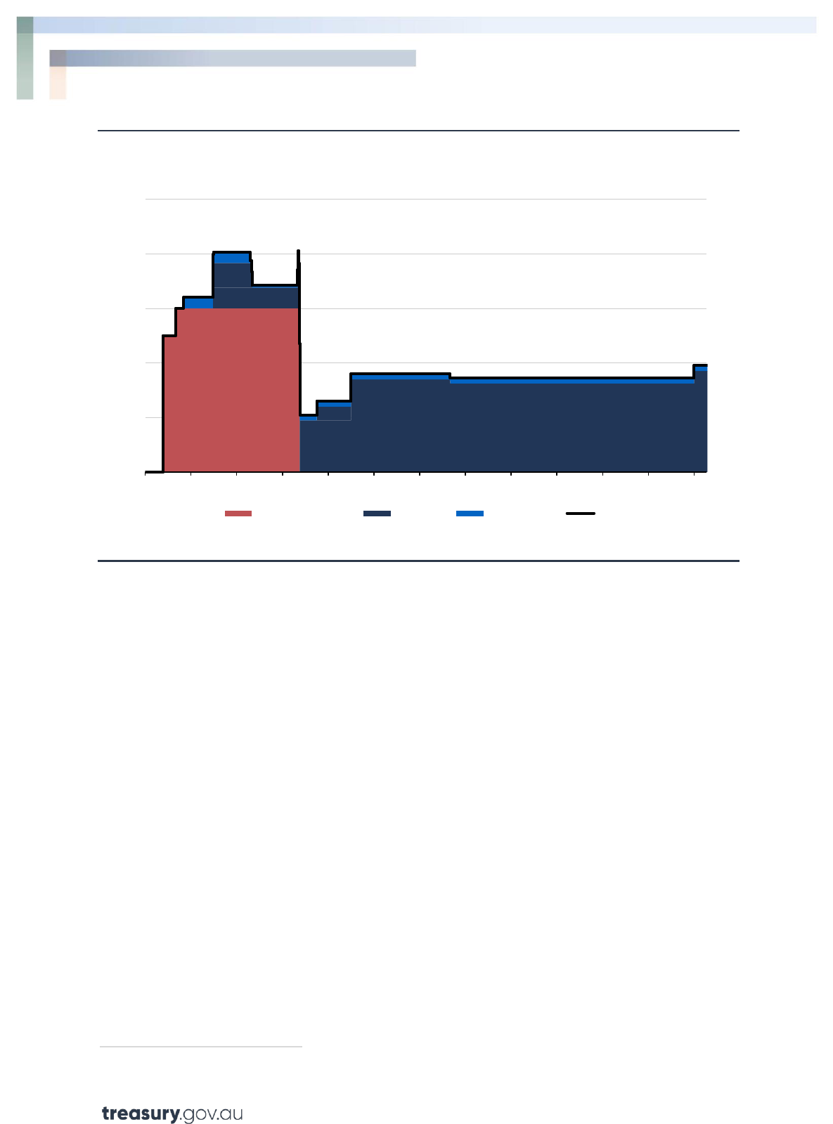
Treasury Round Up | March 2024
Incentives for secondary earners and income support recipients | 65
Chart 6.1 EMTRs for a single person on JobSeeker Payment with no children (2022–23)
Source: Treasury’s CAPITA model
Note: JobSeeker recipient has no children.
However, many income support recipients who face opportunity or capability barriers to employment
will not experience a smooth transition to an income level where they cease receiving payments
because they only have the capacity to work part‑time.
Over 2021, around 67 per cent of JobSeeker Payment recipients exited within 12 months (40 per cent
within 6 months) but those who remain often face barriers that inhibit their capacity to work
full‑time. For example, roughly 43 per cent of JobSeeker Payment recipients have been assessed as
having only partial capacity to work, which means they have an impairment that will prevent them
from working more than 30 hours per week over the next two years.
50
For an individual on the
minimum wage, 30 hours per week, equates to an annual income of around $30,000, which means
they are likely to be subject to high EMTRs.
The example I have discussed illustrates the disincentives many income recipients face to increasing
their hours of work. It does not say anything about the incentives to work related to, or adequacy of,
the level of income support payments. Income support payments are a critical part of Australia’s
welfare system and enable people to buy basic goods they need to support job search and
participation in the labour market. The adequacy of payments will also vary with individual
circumstances. A similar point has been made in discussions about the JobSeeker rate and in
submissions to the White Paper. Although the size of these effects is hard to measure, they are
important considerations for the design of support payments.
50 Department of Social Services, Expanded DSS Demographic Dataset, December 2022.
0
20
40
60
80
100
0 10 20 30 40 50 60 70 80 90 100 110 120
Effective Marginal
Tax Rate (%)
JobSeeker recipient's earned income ($ '000 pa)
JobSeeker Payment Income tax Medicare Levy EMTR

Treasury Round Up | March 2024
Incentives for secondary earners and income support recipients | 66
7 Policy options
If we want to improve incentives for secondary earners and income support recipients then we must
navigate the ‘Iron Triangle’ of means testing. This describes the three‑way trade‑off between the
adequacy of government payments (including for supporting job search), the costs to taxpayers, and
the disincentives for people to get off the payment by earning income.
Transfer payment design
In Australia, incentives and disincentives for secondary earners and income support recipients are
most visible through eligibility for and withdrawal of transfer payments. Therefore, increasing work
incentives for secondary earners or income support recipients, without reducing the payment level,
requires relaxing or removing income‑based means tests.
One option is reducing taper rates. This is the amount a payment is reduced per dollar increase in
income.
Another option to increase incentives to work is to increase the amount of credit that income
support recipients can accumulate through arrangements like Working Credit, which helps smooth
the transition from being on income support to coming off payments. This is particularly important
for those working variable hours. The Government has implemented an option like this for Age
Pensioners and Veterans Pensioners on a temporary basis until 31 December 2023.
Trade-offs – fiscal considerations and the role of the tax system
However, as demonstrated by the Iron Triangle, there are trade‑offs with any changes to current
settings. Any improvement in transfer payment incentives will ultimately have a budgetary cost if
there are no other changes. Given our fiscal challenges over coming decades, any package of changes
will need to be revenue‑neutral in the near term and revenue‑positive in the long term.
Revenue raising is not and should not be the only objective of tax reform. Taxes influence behaviour,
so it is important that any reform adheres to core tax policy design principles, such as the 2009 Henry
Tax Review’s principles of equity, efficiency, and simplicity. This means the tax system should aim to
treat individuals with similar economic capacity in the same way, raise and redistribute revenue at
the least possible economic cost, and be simple to understand.
Australia’s tax system is not always consistent with these principles. For example, it is easier to reduce
tax on income from passive sources than it is for salary and wage income.
There are non‑tax opportunities to make participation incentives clearer to income support recipients
and secondary earners which could help drive participation. Key reports such as the McClure Review
and Henry Tax Review have found that individuals find it difficult to understand the complex
interactions between tax, welfare payments, and additional earnings from work. People are more
likely to rely on rules of thumb and put significant weight on losing benefits such as a Health Care
Card or social housing. These findings have been reinforced by the stakeholder engagement Treasury
has been undertaking for the Employment White Paper.

Treasury Round Up | March 2024
Incentives for secondary earners and income support recipients | 67
8 Conclusion
I have used this speech to highlight one barrier to participation – disincentives to work in current
tax‑transfer settings. Secondary earners face high disincentives to take additional days of work,
particularly the fifth day.
Income support recipients face steep disincentives when working part‑time, which permanently
reduce the returns to work for those who are unable to work full‑time. Addressing these work
disincentives requires making changes to current tax‑transfer settings, and this will have fiscal
consequences in a tight budgetary environment.
Further, for changes to have significant impact, macroeconomic policy must seek to maintain full
employment or close to it. In conditions of higher unemployment, secondary earners may struggle to
increase their participation, and income support recipients are likely to find it more difficult to get
work.
I would like to finish with one obvious point and one point that is often overlooked. The obvious point
is that increasing labour force participation provides financial benefits to workers through wages and
to the Commonwealth through additional revenue and reduced welfare costs.
The point often overlooked is that there are health and wellbeing benefits associated with being
employed. Research finds there are, for most people, clear physical and mental health benefits. For
example, HILDA data shows that working is associated with better mental health and lower rates of
psychological distress. We also know that there are strong intergenerational benefits as children with
parents who work are more likely to work themselves.
Just as the previous employment white papers made substantial contributions to Australian society,
the 2023 Employment White Paper will explore how to extend the benefits of work to people who
face barriers to employment.
But it is critical that any future directions consider system simplicity and fiscal responsibility. This is
another way the 2023 White Paper will, like its predecessors, be a product of its time.
