PowerPoint Presentation

An introduction to image processing using ImageJ

Mark Willett, Imaging and Microscopy Centre,

Centre for Biological Sciences, University of Southampton.

[Shift] + Left click to select and open

everything between two selections in a list

[Ctrl] + Left click to make multiple

individual selections

Drag and drop onto the menu bar to open single or multiple images or stacks

A note on image formats

Images are comprised of pixels, each with an x,y coordinate and an intensity value that gives

the pixel contrast in comparison to adjacent pixels.

The bit-depth of an image is defined by the number of intensity values available to each of

the pixels in an image.

e.g.

Binary = 2 values, (black or white)

8-bit = 256 values. Black (0), white (255) and a scale of 254 grey steps in between

12-bit = 4,096 grey values

16-bit = 65,536 grey values

RGB formats are colour images comprised of 3 channels (red, green and blue) each channel

has independent grey values, usually 8-bit

e.g. an RGB image that has 3 channels x 256 possible values per pixel is 3 x 8-bit = 24-bit

The standard scientific image file format is the uncompressed Tagged Image File Format (.tiff,

.tif) although some microscope manufacturers use their own similar proprietary lossless

formats.

.Tiffs contain an embedded notepad file that contains essential information about the image

such as scaling, laser wavelengths etc (metadata).

Non-scientific file formats such as .jpeg should be avoided as they are “lossy” (some of the

image information is lost because they are compressed to reduce the file size, but are usually

ok for presentations).

It’s usually also best to avoid Windows art packages and non-scientific image viewing and

manipulation packages as they may apply compression to your image and display your image

differently from scientific viewing and analysis packages.

A note on image formats

Viewing image metadata (.tiffs only)

View image metadata by selecting Image>Show Info... Metadata contains

information such as scaling, pixel dimensions, bit depth, fluorescence wavelength

etc.

Some image analysis functions need to use 8-bit image formats (256 grey values)

Change the bit depth using Image>Type.

255

Dynamic range of grey values

Number of pixels

Displayed

black value

Displayed

white value

Distribution of

image intensity

values

The image histogram (8-bit image example)

255

Number of pixels

Maximum pixel value is 80 out of a possible 255. The image is too

dark. This might have been necessary to retain a short exposure

time or reduce photobleaching/phototoxicity of the specimen.

255

Number of pixels

Image is bright but only has

80 steps of intensity

Intensity scaling

When the white value is moved all of the grey values between black and white are re-

scaled so the image appears brighter, however actual pixel values remain unchanged.

Number of pixels

All pixels set to

white

255

Image has been saturated during acquisition. Contrast of all

pixels over 255 is permanently lost

255

Number of pixels

All pixels set to

white

200

Image saturated during processing by incorrect placement of white value

255

Number of pixels

All pixels

set to black

Removes background (and low intensity image information) noise or tell ImageJ

which intensities to send to black and which to white when making a binary image.

Thresholding

Scaling image brightness automatically

Open image “Microtubules 8-bit”. This image does not use the whole dynamic range.

Image>Adjust>Brightness/Contrast, Select ”Auto”. Don’t adjust sliders.

This function moves the displayed white value to the point where 0.4% of pixels are

saturated. All the grey values are then re-scaled and the image appears brighter .

As you can see from the histogram, actual pixel values remain unchanged and intensity

can still be measured if desired.

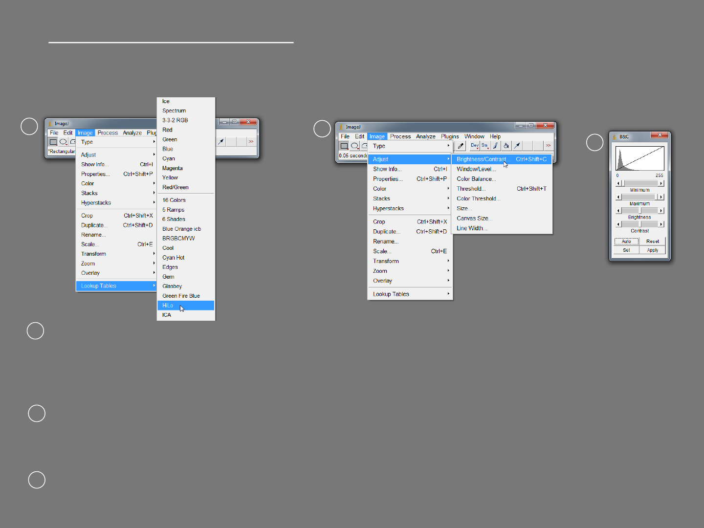
Scaling image brightness manually

Open “Microtubules 8-bit” again. This method also does not change actual pixel

values.

Select Image>Lookup Tables>HiLo and then Image>Adjust>Brightness/Contrast.

Saturated pixels (value of 255) now appear red and pixels with a value of 0 appear

blue.

Adjust the Maximum slider until you get few red pixels and then back it off until they

just disappear.

Adjust the “Minimum” slider until the background turns blue. Click “Apply” then

select Image>Lookup Tables>Grays.

Open image “Peccary hair”

Select Image>Transform>Rotate....

Tick “Preview”. Adjust Angle slider until to

achieve the desired rotation. Click OK.

Rotating images

Cropping

With the image you just rotated, using

the rectangular selection icon, drag a

selection around the area that you

want to keep.

Select Image>Crop

For consistency of size, crop regions can be

stored in the ROI mananger.

Analyze>Tools>ROI Manager...

Calibrating images

Before you can add a scale bar or analyse images, the images have to be calibrated to the

correct measurement units.

Many instruments automatically add spatial calibrations to the image metadata during

acquisition. To check if your images are calibrated look in the top left hand corner of the

image. If your image dimensions are given in pixel units the image has not been

calibrated.

Uncalibrated

Calibrated

If your image is not automatically calibrated by the acquisition software, an image of a

stage micrometer taken at the same magnification as your specimen can be used to

calibrate your images.

(1 small increment on the micrometer = 10 µm)

Open images “calibration image” and

“Uncalibrated image”. Using the line tool,

draw a line of a known distance on the

image of the stage micrometer.

Select Analyze>Set Scale.

Enter the known distance and units in

um. Ticking “Global” applies the

calibration to all images in the Imagej

session.

Manually calibrating images

Adding a scale bar

With your calibrated image open

select Analyze>Tools>Scale Bar.

Select the required width and

position and click “OK”.

Merging images into multichannel 24-bit RGB .tifs

Open images “Blue.tif, Green.tif, Red.tif” and “Brightfield.tif”.

Select Image>Colour>Merge Channels

Select each image into their corresponding colour channels.

Untick “Create composite”, tick “Keep source images” and click “OK”.

Select Image>Colour>Merge Channels

Select Green.tif in the green channel and Brightfield.tif in the grey channel

Untick “Create composite”, tick “Keep source images” and click “OK”.

Splitting multichannel RGB images

Open image “Mitotic cell”.

Select Image>Colour>Split Channels.

Applying pseudocolour to grey images

Using your open grey images split from “Mitotic cell.tif”, Select a channel image by

clicking on it then select Image>Lookup Tables.

Select the correct corresponding colour from the drop down menu.

To return a channel to grey, select “Grays” from the drop down menu.

Stacks

z or t

Individual

images

Stacks are a method of handling multiple related images in one file.

They are often used to handle multiple slices through the vertical z-axis of a specimen

(a z-stack), but are also used to handle sequential images in a time lapse experiment (a t-

stack) or images acquired at different wavelengths (a λ-stack).

Stacks can have up to three dimensions e.g. [x,y],[channels],[z or t or λ].

Stacks with more than three dimensions e.g. {[x,y],[channels],[z]},[t] are called hyperstacks.

View image stacks as a montage

Open z-stack 4EBP1.tif

Select Image>Stacks>Make Montage

Convert stacks to single images

Open z-stack 4EBP1.tif

Select Image>Stacks>Stack to Images

Convert single images to stacks

Using your single images split from z-stack 4EBP1.tif

Select Image>Stacks>Images to Stack

In the pop up window, type something that is in the title of all of the images.

Make a substack or a single slice from a stack into a separate image

Displayed Slice number is shown in the top left hand corner of the stack

Select Image>Stacks>Tools>Make Substack

Enter slice number for a single image, or range if you want to make a substack.

Project a stack to a 2D image

Select Image>Stacks>Z Project….

Select start and finish slices that you want to project and Projection type “Max intensity”

Select regions of interest (ROIs) for measurement using the Rectangular, Polygon, Oval,

Freehand and Line selection tools.

When the cursor is a cross you can click and drag to make your ROI. Placing your cursor in the

middle of your ROI (it changes to an arrow) allows you to move your ROI.

Open image 4E Cisternae.tif

Basic selections and measurements

To set the type of measurement to be made with the ROI, select

Analyse>Set Measurements... and tick the relevant boxes then click “OK”.

Area returns the area within the ROI in the calibrated units

(or pixels

if the image is

uncalibrated).

Mean gray value returns the average grey value inside the ROI.

Integrated density is the average grey value * area inside the ROI.

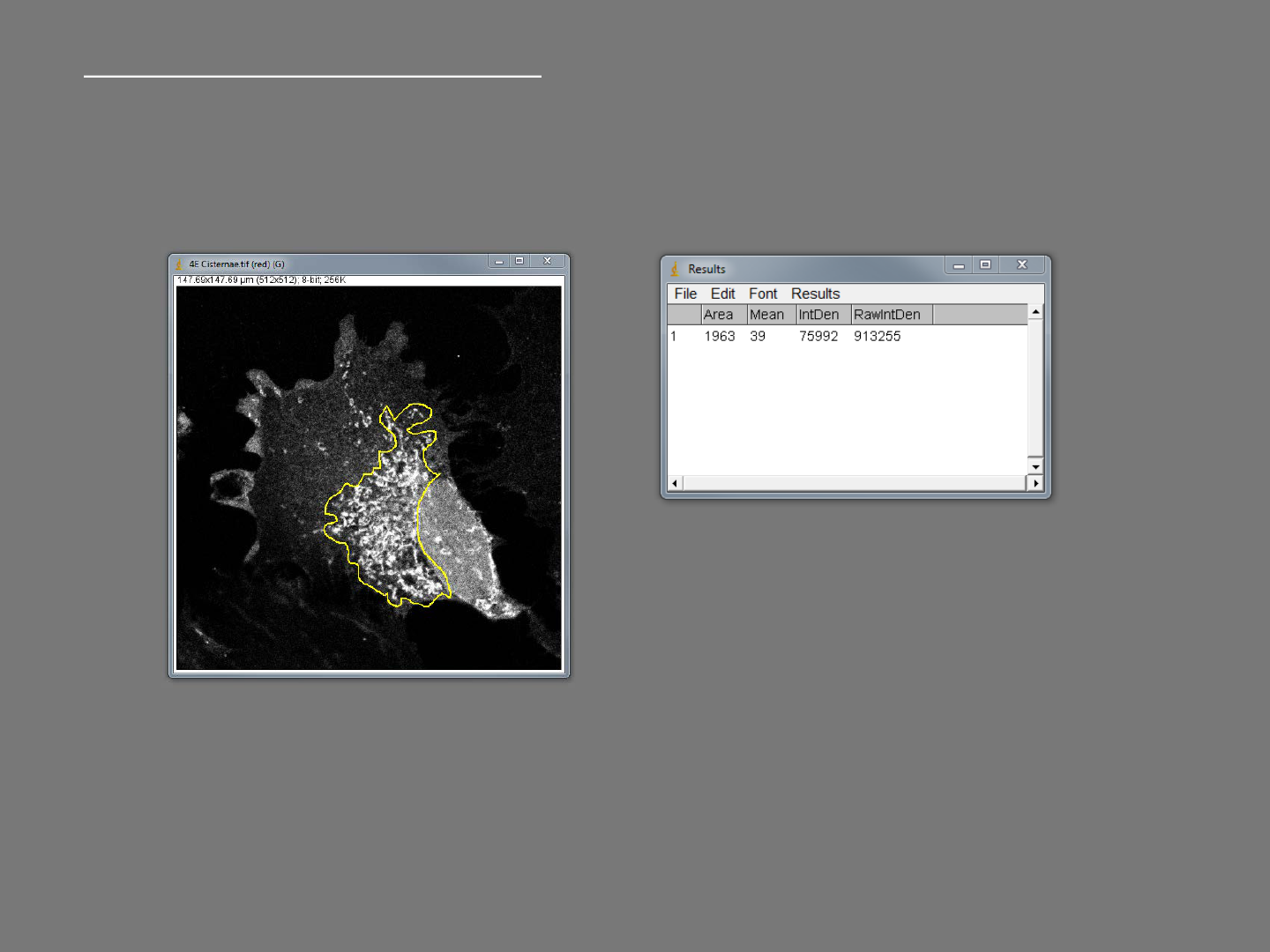
Basic selections and measurements

Press [Ctrl+M] to make the measurement

Draw an ROI on the image using one of the selection tools.

Multiple measurements can be made (select a

new ROI and press [Ctrl+M] again).

You can calculate the mean and standard

deviation of the whole dataset by selecting

Results>Summarize from the Results window.

Results can also be copied and pasted into

Excel for further analysis.

Basic selections and measurements

The ROI manager

Multiple ROIs can be stored and recalled using

the ROI manager.

Select Analyze>Tools>ROI Manager...

To add the current ROI to the ROI manager

click “Add”.

To recall the ROI into any image select it from

the list on the left.

Select More>>Save... On the ROI manager

window to save ROIs for later use.

To change the colour and weight of the ROI

click “Properties” on the ROI manager window.

Background correction

Ideally the grey value for the image background should be as close to 0 as possible

with similar values across the whole image background.

Poor quality or incorrectly configured illumination may cause an uneven background.

Some microscope systems allow grey value “offset” during acquisition, however this

can also be achieved post-acquisition if necessary using several methods:

Rolling Ball – Corrects uneven illumination and preserves low intensity fine specimen

detail.

Thresholding – Subjective and removes low intensity image information as well as

the background.

Background subtraction – Removes low intensity image information as well as the

background. Based on average background intensity, better when quantification is

required.

Background correction - Rolling Ball

This method Imagines a ball or paraboloid rolled around the image. Areas of grey

value large enough for the “ball” to touch to are removed.

This has the advantage over simple background subtraction of preserving low

intensity fine detail in the image and correcting uneven illumination.

Before After

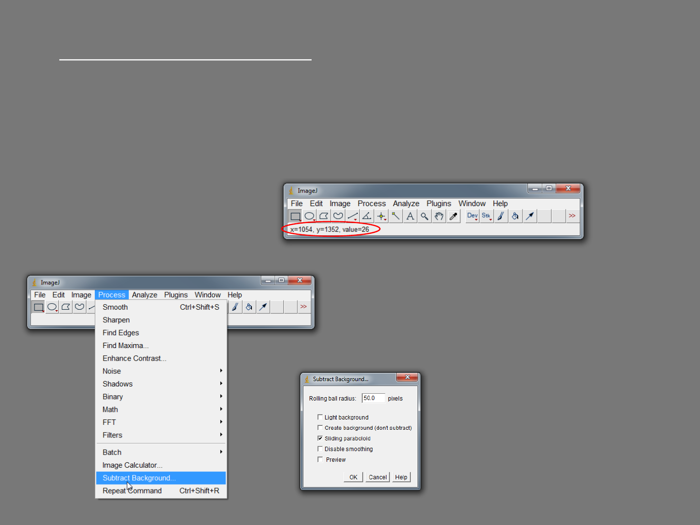
Background correction - Rolling Ball

Open image “Background correction example”. This image has a background

problem as well as uneven illumination, and has a large circular artefact from the

dish that the cells were imaged in.

If you hover the cursor over the image, the grey value of the pixel under the cursor is

displayed on the menu bar.

Select Process>Subtract Background. Tick

“Sliding paraboloid” and choose a “Rolling

ball radius” of 50 pixels and click “OK”.

Background correction - Thresholding

Close your background corrected image without saving and open image “Background

correction example” again.

Select Image>Lookup Tables>HiLo and then Image>Adjust>Brightness/Contrast.

Saturated pixels (value of 255) now appear red and pixels with a value of 0 appear blue.

Adjust the “Minimum” slider until the entire background is blue. All pixels with a value

below the selected threshold (including image information!) will be set to 0. Click “Apply”

then Select Image>Lookup Tables>Grays.

1 2

Background correction - Subtraction

Close your background corrected image without saving and open image “Background

correction example” again.

Select Analyze>Set Measurements and then tick the “Mean gray value” box and click

“OK”.

Select an ROI on an area of background and select Analyze>Measure or use [Ctrl+M]. A

results window should appear with the mean grey value of the pixels within your ROI.

Background correction - Subtraction

Deselect your ROI by clicking on the image or the subtraction will only be applied within

the ROI. Select Process>Math>Subtract and enter your mean background value into the

value field on the window that appears. Click “OK“ or select “Preview”.

Removing noise

Image noise tends to manifest as speckle and can be caused by:

 Electronic variations in imaging detectors.

 Analogue to digital conversion during image acquisition.

 Variations in photon detection, particularly from low signal specimens: “shot noise”.

 High detector gain: “dark noise”.

Speckle can also be caused by contamination such as dust in the sample auto-fluorescing

and by precipitates from stains, so its good practice to wash or flame coverslips and slides

and centrifuge stains prior to use.

Care should be taken when doing noise corrections on images, which may not be suitable

if quantitative measurements are to be made.

Removing noise - outliers

Open image “despeckle 3”. This image is suffering from speckle caused by high detector

gain and also has some large speckles which are probably caused by stain precipitates

reacting with the coverslip coating.

Remove the large bright speckles:

This function replaces a pixel with the median value of the surrounding pixel values if it

deviates from the median by more than the thresholded value. Select “Preview” Reduce

the threshold value until the bright outliers disappear (about 90 in this case). Click “OK”

when finished

Removing noise - speckle

Remove the detector noise:

This function replaces each pixel with the median value of the surrounding 3x3 pixels.

Select Process>Noise>Despeckle.

Use image>Adjust>Brightness/Contrast and the minimum slider to background correct

your image

Open the original image to compare the differences.

Making precise selections – binary selection method

Open image “C elegans lipid store”.

Set the second pulldown menu to “Red”.

Select Image>Adjust>Threshold and threshold the image using the “minimum” slider.

Click “Apply” to make a binary image.

Making precise selections – binary selection method

Select Edit>Selection>Create Selection. An ROI will appear over the binary image

Making precise selections – binary selection method

Select Analyze>Tools>ROI Manager and click “Add”. A new ROI appears in the ROI

manager.

Open the original image “C elegans lipid store”. Select the ROI in the ROI manager, the

ROI will appear on the original image ready for analysis.

Making precise selections – Wand (tracing) tool

The wand (tracing) tool Makes selections

based on grey values when clicked or

dragged across an image.

You can double click the icon to set the tolerance, but it works best

with a thresholded or binary image.

Open “Mitotic cell.tif (red)”.

Select Image>Adjust>Threshold and threshold the image.

Do not click “Apply”.

Select the Wand (tracing) tool. Click

and drag to make the selection

then add your selection to the ROI

manager.

or reset the threshold

And make your

measurements immediately

Making precise selections – Wand (tracing) tool