Instance Segmentation of Indoor Scenes
using a Coverage Loss
Nathan Silberman, David Sontag, Rob Fergus
Courant Institute of Mathematical Sciences, New York University
Abstract. A major limitation of existing models for semantic segmen-
tation is the inability to identify individual instances of the same class:
when labeling pixels with only semantic classes, a set of pixels with the
same label could represent a single object or ten. In this work, we in-
troduce a model to perform both semantic and instance segmentation
simultaneously. We introduce a new higher-order loss function that di-
rectly minimizes the coverage metric and evaluate a variety of region
features, including those from a convolutional network. We apply our
model to the NYU Depth V2 dataset, obtaining state of the art results.
Keywords: Semantic Segmentation, Deep Learning
1 Introduction
Semantic segmentation models have made great strides in the last few years.
Following early efforts to densely label scenes [1], numerous approaches such as
reasoning with multiple segmentations [2], higher-order label constraints [3] and
fast inference mechanisms [4] have advanced the state of the art considerably.
One limitation in all of these methods, however, is their inability to differentiate
between different instances of the same class. This work introduces a novel algo-
rithm for simultaneously producing both a semantic and instance segmentation
of a scene. More specifically, given an image, we produce both a semantic label
for every pixel and an instance label that differentiates between two instances
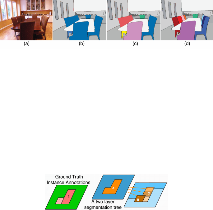
of the same class, as illustrated in Fig. 1.
The ability to differentiate between instances of the same class is important
for a variety of tasks. In image search, one needs to understanding instance
information to properly understand count-based searches: “three cars waiting at
a light” should retrieve different results from “a single car waiting at the light”.
Robots that interact with real world environments must understand instance
information as well. For example, when lifting boxes a robot needs to distinguish
between a single box and a stack of them. Finally, being able to correctly infer
object instances drastically improves performance on high level scene reasoning
tasks such as support inference [5] or inferring object extent [6] [7].
Unfortunately, searching over the space of all semantic and instance segmen-
tations for a given image is computationally infeasible. Like many previous works
in semantic segmentation [8] [4] [9], we use a heuristic to limit the search space
by first performing a hierarchical segmentation of the image. This produces a
set of nested segments that form a tree, referred to as a segmentation tree.
2 Nathan Silberman, David Sontag, Rob Fergus
Our goal during inference is to (a) find the best non-overlapping subset of
these segments such that each pixel is explained by a single region from the
tree – referred to as cutting the segmentation tree – and (b) each selected region
is labeled with a semantic label denoting the class and instance ID (e.g. chair
#2). The inference procedure finds the cut through the segmentation tree that
maximizes these two objectives. During learning, we will seek to maximize the
Coverage Score [10], a measure of how similar two segmentations are, between our
inferred semantic/instance segments and those produced by human annotators.
Fig. 1. An illustration of the limits of semantic segmentation: (a) the input image. (b)
a perfect semantic segmentation; note all of the chair pixels are labeled blue. (c) a naive
instance segmentation in which all connected components of the same class are consid-
ered separate instances of the chair class. (d) a correct instance segmentation, which
correctly reasons about instances within contiguous segments and across occlusions.
While at a high level this approach is similar to many semantic segmentation
methods, two main factors complicate the joint learning of semantic-instance
segmentation models using segmentation trees:
The Ground Truth Mapping Problem: When using a reduced search space,
such as one provided by a given hierarchical segmentation, it is extremely rare
that the exact ground truth regions are among the set of bottom-up proposed
regions, due to mistakes made at detecting object boundaries. Therefore, during
training, we must be able to map the human-provided labels to a set of surrogate
labels, defined on the set of proposed regions.
Fig. 2. Computing the best possible set of instances that overlap with the ground truth
cannot be computed independently per ground truth region. For example, ground truth
region 2 best overlaps with proposed region A and ground truth region 1 best overlaps
with proposed region B. But both proposed regions A and B cannot be selected at the
same time because they overlap.
Obtaining these surrogate labels is problematic for semantic-instance seg-
mentation. The constraint that the regions must not non-overlap means the best
possible subset of regions cannot be computed independently as the inclusion of
Courant Institute of Mathematical Sciences, New York University 3
one region may exclude the use of another (see Figure 2). Therefore, computing
the ‘best possible’ instance segmentation with respect to a segmentation tree is
an optimization problem in its own right.
Identifying a Good Loss Function: In semantic segmentation, it is easy to
penalize mistakes: a region is either assigned the correct or incorrect label. In our
setting, we require a more continuous measure, since an inferred region might
not exactly match the ‘best’ region, but it might be extremely close (e.g. differ-
ing by a single pixel). While a continuous higher order loss function for binary
segmentation has previously been proposed [11], it cannot handle the multiple
ground truth regions encountered in complex scenes.
Our Contributions: To summarize, we introduce:
1. A novel and principled structured learning scheme for cutting segmentation
trees.
2. A new higher order loss, appropriate for semantic-instance segmentation,
which directly optimizes the Coverage score.
3. An efficient structured learning algorithm based on block-coordinate Frank
Wolfe and a novel integer linear program for loss-augmented inference
4. A quantitative analysis of the use of features from state-of-the-art convolu-
tional networks and their application to segmenting densely labeled RGB-D
scenes.
2 Related Work
For certain classes of objects, such as cars or pedestrians, instance information
can be recovered from detectors. While the state of the art in object localization
[12] has improved dramatically, they perform best with large objects that occupy
a significant portion of the image plane and struggle when the objects exhibit
large amounts of occlusion. Furthermore, they do not in themselves produce a
segmentation.
Motivated by the observation that a single segmentation of an image is un-
likely to produce a perfect result, numerous approaches [13] [14] [15] [16] make
use of multiple segmentations of an image. These approaches differ in how they
use the various segmentations and whether the regions proposed are strictly hi-
erarchical or structureless. Starting with [13], various efforts [3] [17] have used
multiple independent segmentations in a pixel labeling task. While these works
are ultimately interested in per-pixel semantic labels, ours reasons about which
regions to select or ignore and outputs both semantic and instance labels.
Several works [18] [19] use a structureless bag of regions to perform segmen-
tation in which inference comprises of a search for the best non-overlapping set
of regions that respects object boundaries. However, neither work uses seman-
tics for reasoning. Rather than use arbitrary or structureless regions as input,
an increasing number of approaches [2] [8] [4] [9] have been introduced that
utilize hierarchical segmentations to improve semantic segmentation. Like our
approach, these models are trained to cut a segmentation tree. The major differ-
ence between these works and our own is that the product of these algorithms
do not differentiate between instances of objects.
4 Nathan Silberman, David Sontag, Rob Fergus
Higher order losses for segmentation have also been previously explored. Tar-
low et al. [11] introduce the Pascal Loss which smoothly minimizes the overlap
score [20] of a single foreground/background segmentation. The Pascal Loss is
closely related to the Coverage loss. A crucial difference between the two is that
in the case of Pascal Loss, the best overlapping region is specified a priori (there
is only one region, the foreground), whereas in the Coverage Loss, the best over-
lapping region can only be computing by jointly reasoning over every proposed
region.
3 Segmentation Trees
Because the space of all semantic-instance segmentations is so large, we must
limit the solution space to make the problem tractable. Like previous work in
semantic segmentation [2] [8] [4] [9], we make use of hierarchical segmentations,
referred to as segmentation trees, to limit the search space to a more manageable
size. A set of regions or segments S = {s
1
, . . . , s
R
} forms a valid segmentation
tree T = {S, P } for an image I if it satisfies the following constraints:
Completeness: Every pixel I
i
is contained in at least one region of S.
Tree Structure: Each region s
i
has at most one parent: P (s
i
) ∈ {∅, s
j
}, j 6= i
Strict Nesting: If P (s
i
) = s
j
, then the pixels in s
i
form a strict subset of s
j
A cut T (A) of the tree selects a subset S
A
⊂ S of segments that form a planar
segmentation, a map M : I
i
7→ Z from each pixel I
i
to exactly one region. The
goal of this work is to take as input a segmentation tree and cut it such that
the resulting planar segmentation is composed of a set of regions, each of which
corresponds to a single object instance in the input image.
During training, we will make use of two types of segmentation trees: stan-
dard segmentation trees and Biased Segmentation Trees.
3.1 Standard Segmentation Trees
We use the term standard segmentation tree to refer to a hierarchical segmen-
tation created by iteratively merging similar regions based on local boundary
cues until a pre-specified stopping criteria is met. While various schemes [21]
[10] have been introduced to perform this operation, we use the method of [22].
To summarize, given an image I of size H × W , we begin by producing a grid
L
H,W
where each pixel corresponds to a node in the graph and edge weights
between neighboring pixels indicate the probability that each neighboring pair
of pixels are separated by a region boundary. As in [22], the edge weights are
computed by first extracting gPb features [23] and calculating the Ultrametric
Contour Map (UCM). To create a segmentation at a particular scale, edges with
weights lower than some threshold are removed and the induced regions are the
connected components of the resulting graph. This process is repeated with var-
ious thresholds to create finer or coarser regions. The unique superset of regions
produced by the various thresholded region maps form a tree T such that each
region is represented as a node and any pair of region r
i
, r
j
are the children of
region r
k
if r
i
and r
j
are both sub-regions of r
k
.
Courant Institute of Mathematical Sciences, New York University 5
3.2 Biased Segmentation Trees
Using only standard segmentations trees, one cannot properly evaluate whether
the limitation of a particular tree cutting algorithm is the quality of the regions
it has to select from or the capacity of the model itself. To separate these sources
of error, we need a tree that contains, as a possible cut, a specified planar seg-
mentation, which we refer to as a biased segmentation tree. In particular, we
wish to take as input a ground truth planar segmentation provided by a human
labeler and create a segmentation tree that contains the ground truth regions
as a possible cut. With such trees, we are able to properly evaluate tree-cutting
model errors independant of segmentation tree creation errors.
To create biased segmentation trees, we first threshold the UMC to obtain a
base set of regions. Next, we split these regions further by taking the intersection
of every ground truth region with the segmented regions. Edge weights for newly
introduced boundaries are computed using the average gPb values for each pixel
along each boundary. Any boundary aligned with a ground truth edge is given
a weight of 0. Next, we use the same algorithm as in Section 3.1 to produce
several fine segmentations culminating in the ground truth segmentation. Finally,
a coarser set of regions is obtained by repeating this process starting from the
ground truth regions. In this final step, any boundary inside a ground truth
region is given a weight of 0 and any boundary aligned with a ground truth
region is computed by averaging the gPb values along the boundary pixels.
4 Cutting Instance Segmentation Trees
Given an image and a segmentation tree, our goal is to find the best cut of the
tree such that each of the resulting regions corresponds to a single instance of
an object and is labeled with the appropriate semantic class.
Let a cut of the tree be represented by {A : A
i
∈ {0, 1}, i = 1..R}, a vector
indicating whether or not each of the R regions in the tree are selected. Let
{C : C
i
∈ {1..K}, i = 1..R} be a vector indicating the semantic class (out of
K classes) of each region. Finally let y = {A, C} be the combined output of
semantic labels and region instances.
4.1 Model
We perform structured prediction by optimizing over the space Y of region selec-
tions and semantic class assignments for a given segmentation tree. Formally, we
predict using y
∗
= arg max
y∈Y
w
T
φ(x, y), where x represents the input image, y
encapsulates both the region selection vector A and class assignments C, and w
represents a trained weight vector. φ is a feature function on the joint space of
x and y such that w
T
φ(x, y) can be interpreted as measuring the compatibility
of x and y. w
T
φ(x, y) can be decomposed as follows:
w
T
reg
φ
reg
(x, y) +
K
X
k=1
w
T
sem:k
φ
sem:k
(x, y) + w
T
pair
φ
pair
(x, y) + φ
tree
(y)

6 Nathan Silberman, David Sontag, Rob Fergus
The generic region features encode class-agnostic appearance features of
selected regions: φ
reg
(x, y) =
P
R
i=1
f
reg
i
[A
i
= 1], where f
reg
i
are region features
extracted from region i and [. . .] is the indicator function. The semantic com-
patibility features capture class-specific features of each region: φ
sem:k
(x, y) =
P
R
i=1
f
sem
i
[A
i
= 1∧C
i
= k], where k is the semantic class and f
sem
i
are semantic
features extracted from region i.
The pairwise features φ
pair
(x, y) are given by
P
ij∈E
f
pair
ij
[A
i
= 1 ∧ A
j
= 1],
where E is the set of all adjacent regions and f
pair
ij
are pairwise features extracted
along the boundary between regions i and j. Finally, the tree-consistency
function φ
tree
(y) ensures that exactly one region along every path from the leaf
nodes to the root node of the tree is selected:
φ
tree
(y) =
X
γ∈Γ
−∞
1 6=
X
i∈γ
1[y.A
i
= 1]
, (1)
where Γ is the set of paths in the tree from the leaves to the root.
4.2 Learning
Let D = {(x
(1)
, y
(1)
), ...(x
(N)
, y
(N)
)} be a dataset of pairs of images and labels
where y
(i)
= {A, C} comprises the best assignment (Section 6) of segments from
the pool and semantic class labels for image i. We use a Structured SVM [24]
formulation with margin re-scaling to learn weight vector w:
min
w, ξ≥0
1
2
w
T
w +
λ
N
N
X
i=1
ξ
i
(2)
s.t. w · [φ(x
(n)
, y
(n)
) − φ(x
(n)
, y)] ≥ ∆(y, y
(n)
) − ξ
n
∀n, y ∈ Y
where ξ
i
are slack variables for each of the training samples 1..N , and λ is a reg-
ularization parameter. The definition of the loss function ∆(y, y
(n)
) is discussed
in more detail in Section 5.
4.3 Inference
We first show how the inference task, arg max
y∈Y
w
T
φ(x, y), can be formulated
as an integer linear program. To do so, we introduce binary variable matrices to
encode the different states of A and C and auxiliary vector variables p to encode
the pairwise states. Let a ∈ B
R×2
encode the states of A such that a
i,0
= 0
indicates that region i is inactive and a
i,1
= 1 indicates that region i is active.
Let c
i,k
encode the states of C such that c
i,k
= 1 if C
i
= k and 0 otherwise.
Finally, let p ∈ B
E×1
be a vector which encodes whether any neighboring pair
of regions are both selected where E is the number of neighboring regions. Our

Courant Institute of Mathematical Sciences, New York University 7
integer linear program is then:
arg max
a,c,p
R
X
i=1
θ
r
i
a
i,1
+
R
X
i=1
K
X
k=1
θ
s
i,k
c
i,k
+
X
ij∈E
θ
p
ij
p
ij
(3)
s.t. a
i,0
+ a
i,1
= 1 (4)
K
X
k=0
c
i,k
= 1, a
i,0
= c
i,0
∀ i ∈ R (5)
X
i∈γ
a
i,1
= 1 ∀ γ ∈ Γ (6)
p
ij
≤ a
i,1
, p
ij
≤ a
j,1
, a
i,1
+ a
j,1
− p
ij
≤ 1 ∀ i, j ∈ E (7)
with generic region costs θ
r
i
= w
T
reg
f
reg
i
, semantic compatibility costs θ
s
i,k
=
w
T
sem:k
f
reg
i
and pairwise costs θ
p
ij
= w
T
pair
f
pair
ij
.
Equation 4 ensures that each region is either active or inactive. Equation
5 ensures that each region can take on at most a single semantic label (or no
semantic label if the region is inactive). Equation 6 ensures that exactly one
region in each of the paths of the tree (from each leaf to most coarse node) is
active. Equation 7 ensures that the auxiliary pairwise variable p
ij
is on if and
only if both regions i and j are selected.
When there are no pairwise features we can give an efficient dynamic pro-
gramming algorithm to exactly solve the maximization problem, having running
time O(RK). When pairwise features are included, this algorithm could be used
together with dual decomposition to efficiently perform test-time inference [25].
However, the integer linear program formulation is particularly useful for loss-
augmented inference during learning (see Section 5.1).
5 Coverage Loss
Let G = {r
G
1
, ...r
G
|G|
} be a set of ground truth regions and S = {r
S
1
, ...r
S
|S|
} be
a set of proposed regions for a given image. For a given pair of regions r
j
and
r
k
, the overlap between them is defined using the intersection over union score:
Overlap(r
j
, r
k
) = (r
j
∩ r
k
)/(r
j
∪ r
k
). The weighted coverage score [10] measures
the similarity between two segmentations:
Coverage
weighted
(G, S) =
1
|I|
|G|
X
j=1
|r
G
j
| max
k=1..|S|
Overlap(r
G
j
, r
S
k
). (8)
where |I| is the total number of pixels in the image and |r
G
j
| is the number
of pixels in ground truth region r
G
j
. We define the Coverage Loss function to be
the amount of coverage score unattained by a particular segmentation:
∆
W
1
(y, ¯y) =
1
|I|
|G|
X
j=1
|r
G
j
|
1 − max
k:
¯
A
k
=1
Overlap(r
G
j
, r
S
k
)
(9)
8 Nathan Silberman, David Sontag, Rob Fergus
where ¯y is a predicted cut of the segmentation tree and
¯
A ∈ B
|S|×1
the
corresponding vector indicating which regions are selected.
5.1 Integer Program Formulation with Loss Augmentation
During training, most structured learning algorithms [26] [27] need to solve the
loss augmented inference problem, in which we seek to obtain a high energy
prediction that also has high loss:
y
∗
= arg max
¯y∈Y
∆(y
(i)
, ¯y) + w
T
φ(x, ¯y) (10)
To solve the loss augmented inference problem, we introduce an additional
auxiliary matrix o ∈ B
G×R
where G represents the number of ground truth
regions and R represents the number of regions in the tree. The variable o
gj
will
be 1 if region r
j
is the argmax in (9) for the ground truth region g (specified by
y
(i)
), and 0 otherwise. To ensure this, we add an additional set of constraints:
o
gi
≤ a
i,1
∀ g ∈ G, ∀i ∈ R (11)
R
X
i=1
o
gi
= 1 ∀ g ∈ G (12)
o
gi
+ a
j,1
≤ 1 ∀g ∈ G, i, j ∈ R s.t. Overlap(s
g
, s
j
) > Overlap(s
g
, s
i
) (13)
Equation (11) ensures that a prediction region i can only be considered the max-
imally overlapping region with ground truth region g if it is a selected region.
Equation (12) ensures that every ground truth region is assigned exactly 1 over-
lap region. Finally, Equation (13) ensures that prediction region i can only be
assigned the maximal region of g if and only if no other region j that has greater
overlap with g is active.
The ILP objective is then altered to take into account the coverage loss:
arg max
a,c,p,o
R
X
i=1
θ
r
i
a
i,1
+
R
X
i=1
K
X
k=1
θ
s
i,k
c
i,k
+
X
ij∈E
θ
p
ij
p
ij
+
G
X
g=1
R
X
i=1
θ
o
gi
o
gi
(14)
where θ
o
gi
= Overlap(r
G
g
, r
S
s
)−Overlap(r
G
g
, r
S
i
) encodes the loss incurred if region
i is selected where r
S
s
is the region specified by the surrogate labeling with the
greatest overlap with ground truth region g.
6 Solving the Ground Truth Mapping Problem
Because the ground truth semantic and instance annotations are defined as a
set of regions which are not among our segmentation tree-produced regions, we
must map the ground truth annotations onto our segmented regions in order to
learn. To do so, we build upon the ILP formulation described in the previous
section.
Courant Institute of Mathematical Sciences, New York University 9
Formally, given a ground truth set of instance regions G = {r
g
1
, ...r
g
R
G
} and
a proposed tree of regions S = {r
1
, ...r
R
P
}, the cut of the tree that maximizes
the weighted coverage score is given by the following ILP:
arg min
a,o
G
X
g=1
R
X
i=1
θ
o
gi
o
gi
subject to a
i,0
+ a
i,1
= 1 ∀i ∈ R,
P
i∈γ
a
i,1
= 1 ∀γ ∈ Γ , and Equations (11),(12),
and (13).
6.1 Learning with Surrogate Labels
When the segmentation trees contain the ground truth regions as a possible cut,
the minimal value of the Coverage Loss (Equation 9) is 0. However, in practice,
segmentation trees provide a very small sample from the set of all possible regions
and it is rare that the ground truth regions are among them. Consequently, we
must learn to predict a set of surrogate labels {z
(1)
, ..., z
(N)
} instead.
We modify the loss used in training to ensure that the magnitude of the
surrogate loss of a prediction ¯y
i
is defined relative to the best possible cut z
(i)
:
∆
W
2
(z
(i)
, ¯y) = ∆
W
1
(y
(i)
, ¯y) − ∆
W
1
(y
(i)
, z
(i)
) (15)
Note that the first term in the loss can be pre-computed and has the effect of
scaling the loss such that the margin requested during learning is defined with
respect to the best attainable cut in a given segment tree. It should be clear
then when y
(i)
= z
(i)
, that ∆
W
2
= ∆
W
1
.
7 Convolutional Network Features for Dense
Segmentation
While Convolutional Neural Networks (CNNs) have shown impressive perfor-
mance in Classification [28] and Detection [12] tasks, it has not yet been demon-
strated that CNN features improve dense segmentation performance. Recently
[29] showed how to use a pretrained convolutional network to improve the rank-
ing of foreground/background segmentations on the PASCAL VOC dataset. It is
unclear, however, whether a similar scheme can be successfully applied to densely
labeled scenes, where many of the images can only be identified via contextual
cues. Furthermore, because CNNs are generally trained on RGB data (no RGBD
data exists with enough labeled examples to properly train these deep models) it
is unclear whether CNN features provide an additional performance boost when
combined with depth features. To address these questions, we compare state of
the art hand-crafted RGB+D features with features derived from the aforemen-
tioned CNN models, as well as combinations of the two feature sources. As in
[29], we extract CNN-based region features as follows: for each arbitrarily shaped
region, we first extract a sub-window that tightly bounds the region. Next, we
10 Nathan Silberman, David Sontag, Rob Fergus
feed the sub-window to the pre-trained network of [28]. We treat the activations
from the first fully connected hidden layer of the model as the features for the
region. While we experimented with using the final pooled convolutional layer
and the second fully connected layer, we did not observe a major difference in
performance when using these alternative feature sources.
Because a particular sub-window may contain multiple objects, there exists
an inherent ambiguity with regard to which object in a sub-window is being
classified by the CNN. To address this ambiguity, we experimented with three
types of masking operations performed on each sub-window before the CNN
features were computed. Firstly, we perform no masking (Normal Windows).
Secondly, we blur the subwindow (Mask Blurred Windows) with a blur kernel
whose radius increases with respect to the euclidean distance from the region
mask. This produces a subwindow that appears focused on the object itself.
Finally, we use the masking operation from [29] (Masked Windows) in which
any pixels falling outside the mask are set to the image means so that the
background regions have zero value after mean-subtraction.
We additionally experiment with a superset of region features from [30] and
[5] as well as compare the convolutional network features to Sparse Coded SIFT
features from [31]. Our pairwise region features are a superset of pairwise region
and boundary features from [30] [5].
8 Experiments
To evaluate our instance-segmentation scheme, we use the NYU Depth V2 [5]
dataset. While datasets like Pascal [20], Berkeley [32], Stanford Backgound [33]
and MSRC [1] are frequently used to evaluate segmentation tasks, Stanford Back-
ground and MSRC do not provide instance labels and the Berkeley dataset pro-
vides neither semantic nor instance labels. Pascal only contains a few segmented
objects per scene, mostly at the same scale. Conversely the NYU Depth dataset
has densely labeled scenes with instance masks for objects of highly varying size
and shape.
While the original NYU V2 dataset has over 800 semantic classes, we mapped
these down to 20 classes: cabinet, bed, table, seating, curtain, picture, window,
pillow, books, television person, sink, shelves, cloth, furniture, wall, ceiling, floor,
prop and structure. We use the same classes for evaluating both the CNN features
and the semantic instance segmentation.
8.1 Evaluating Segmentation Tree Proposal Methods
While numerous hierarchical segmentation strategies have been proposed, it has
not been previously possible to estimate the upper bound coverage score of a
particular segmentation tree. Our loss formulation addresses this by allowing us
to directly measure the Coverage upper bound (CUB) scores achievable by a par-
ticular hierarchical segmentation. We evaluate several hierarchical segmentation
proposal schemes in Table 8.1 by computing for each the surrogate labels that
maximize the weighted coverage score. Unsurprisingly the depth signal raises

Courant Institute of Mathematical Sciences, New York University 11
the CUB score. [30] outperforms [5] both in terms of CUB score and requires far
fewer regions. [21] and [10] both achieve the same weighted CUB scores but [21]
is a bit more efficient requiring fewer regions. We use the method from [30] for
all subsequent experiments.
Input Algorithm Weighted CUB Average Number of Regions
RGB Hoiem et al [10] 50.7 117.7 ± 36.7
RGB Zhile and Shakhnarovich [21] 50.7 102.4 ± 56.4
RGB+D Silberman et al (RGBD) [5] 64.1 210.0 ± 106.0
RGB+D Gupta et al [30] 70.6 62.5 ± 26.6
Table 1. Segmentation results on the testing set.
8.2 Evaluating CNN Features
To evaluate the CNN features, we used the ground truth instance annotations
from the NYU Depth V2 dataset. By evaluating on the ground truth regions,
we can isolate errors inherent in evaluating poor regions from the abilities of
the descriptor as well as avoid the ground truth mapping problem for assigning
semantic labels. To prepare the inputs to the CNN we perform the following op-
erations: For each instance mask in the dataset (a binary mask for a single object
instance), we compute a tight bounding box around the object plus a small mar-
gin (10% of the height and width of the mask). If the bounding box is smaller
than 140×140, we use a 140×140 bounding box and upsample to 244×244. Oth-
erwise, we rescale the image to 244 × 244. During training, we use each original
sub-window and its mirror image at several scales (1.1, 1.3, 1.5, 1.7). Finally, we
ignore regions whose original size is smaller than 20×20. We computed a random
train/val/test split using the original 1449 images in the dataset of equal sizes.
After performing each of the aforementioned masking operations and comput-
ing the CNN features from each subwindow, we normalize each output feature
from the CNN by subtracting the mean and dividing by the variance, computed
across the training set. We then train a L2-regularized logistic regressor to pre-
dict the correct semantic labels of each instance. The regularization parameters
were chosen to maximize accuracy on the validation set and are found in the
supplementary material.
As shown in Table 2, the CNN features perform surprisingly well, with
Masked Windows computed on RGB only beating both RGBD Features and
the combination of sparse coded SIFT and RGBD Features. Our Mask-Blurring
operation does not do as well as Masking, with the combination of RGBD Fea-
tures and CNN Features extracted from Masked regions performing the best.
8.3 Segmentation
To evaluate our semantic/instance segmentation results, we use the semantic
and instance labels from [5]. We train and evaluate on the same train/test split

12 Nathan Silberman, David Sontag, Rob Fergus
Features Accuracy Conf Matrix Mean Diagonal
Normal Windows 48.8 23.5
Mask-Blurred Windows 56.6 36.8
Masked Windows [29] 60.8 42.3
RGBD Features [5] 59.9 32.1
Sparse Coded Sift + RGBD Features [31] 60.3 34.4
Unblurred Windows + RGBD Features 60.3 38.0
Mask-Blurred Windows + RGBD Features 63.1 46.1
Masked Windows + RGBD Features 64.9 46.9
Table 2. A comparison on region-feature descriptors on ground truth regions.
as [5] and [34]. We computed the surrogate labels using the weighted coverage
loss and report all of the results using the weighted coverage score. To train
our model, we used the Block Coordinate Frank Wolf algorithm [27] for solving
the structured SVM optizmiation problem, and the Gurobi[35] ILP solver for
performing inference. Loss augmented inference takes several seconds per image
whereas inference at test time takes half a second on average. The difference in
speed is due to the addition of the overlap matrix (Section 5.1) used to implement
loss augmented inference at training time.
Evaluating Semantic-Instance Segmentation Results
We evaluate several different types of Semantic-Instance Segmentation models.
The model SEG Trees, SIFT Features uses the standard segmentation trees
with Sparse Coded SIFT features, SEG Trees, CNN Features uses standard
segmentation trees and CNN Features using the Masking strategy, SEG + GT
Trees, CNN Features uses the CNN features as well but also trains with a set
of height-1 trees created from the ground truth instance maps. Since these height-
1 trees are by definition already segmented, during training we use the Coverage
Loss for the SEG Trees and Hamming Loss on the semantic predictions for the
GT Trees. The last model we evaluated, GT-SEG Trees, CNN Features, is
a model trained on segmentation trees biased by the ground truth.
As shown in Table 3 our model achieves state of the art performance in
segmenting the dense scenes from the NYU Depth Dataset. While the use of
SIFT features makes a negligible improvement with regard to previous work,
using convolutional features provides almost a 1% improvement. SEG + GT
Trees, CNN Features, which was trained to minimize coverage loss on the
SEG trees and semantic loss on the ground truth performs slightly better. The
addition of the GT trees to the training data acts as a regularizer for the semantic
weights on the high dimensional CNN features by requiring that the weights are
both useful for finding instances of imperfectly segmented objects and correctly
labeling objects if a perfect region is made available. Qualitative results for this
model are shown in Fig. 8.3 along with a comparison to [34]. As these figures
illustrate, the model performs better on larger objects in the scene such as the

Courant Institute of Mathematical Sciences, New York University 13
couch in row 1, and the bed in row 4. Like [34] however, it struggles with smaller
objects such as the clutter on the desk in row 5.
Finally GT-SEG Trees, CNN Features is a model trained on segmenta-
tion trees biased by the ground truth. This model achieves a coverage score of
87.4% which indicates that while our model shows improvement over previous
methods at instance segmentation, it still does not achieve a perfect coverage
score even when the ground truth is available as a possible cut.
Algorithm Weighted Coverage
Silberman et al [5] 61.1
Jia et al [34] 61.7
Our Model - SEG Trees, SIFT Features 61.8
Our Model - SEG Trees, CNN Features without Pairwise terms 62.4
Our Model - SEG Trees, CNN Features 62.5
Our Model - SEG + GT Trees, CNN Features 62.8
Our Model - GT-SEG Trees, CNN Features 87.4
Table 3. Segmentation results on the NYU Depth V2 Dataset
Evaluating the Loss function
To evaluate the effectiveness of using the Coverage Loss for instance segmen-
tation, we use the same model but vary the loss function used to minimize the
structural SVM. We compare against using the hamming loss. We use the use
regularization parameter
1
for both experiments.
Loss Function Weighted Coverage
Hamming Loss 61.4
Weighted Coverage Loss 62.5
Table 4. Evaluating the use of the Coverage Loss
9 Conclusions
In this work, we introduce a scheme for jointly inferring dense semantic and
instance labels for indoor scenes. We contribute a new loss function, the Cover-
age Loss, and demonstrate its utility in learning to infer semantic and instance
labels. While we can now directly measure the maximum achievable coverage
score given a set of regions, it is not yet clear whether this upper bound is ac-
tually attainable. While a particular cut of a segmentation tree may maximize
the coverage score, it may be information theoretically impossible to find a gen-
eralizing model as different humans may disagree on the best surrogate labels,
just as they may disagree on the best ground truth annotations. Furthermore,
while our structured learning approach was applied to segmentation trees, it
can be similarly applied to an unstructured ”soup” of segments. In practice, we
1
λ = .001

14 Nathan Silberman, David Sontag, Rob Fergus
Fig. 3. Random test images from the NYU Depth V2 dataset, overlaid with segmen-
tations. 1st column: ground truth. 2nd column: segmentations from Jia et al [34]. 3rd
colmun: our segmentations. 4th column: semantic labels, produced as a by-product of
our segmentation procedure.
found that such an unstructured set of segments did not increase performance
but instead slowed inference. This is due to the fact that the requirement that
no two selected segments overlap can be efficiently represented by a small set of
constraints when using segmentation trees where a ”soup” of segments requires
a very large number of non-overlap constraints. One limitation of our segmen-
tation tree formulation is the inability of the model to merge instances which
are non-neighbors in the image plane. We hope to tackle this problem in future
work.
Acknowledgements: The authors would like to acknowledge support from
ONR #N00014-13-1-0646, NSF #1116923 and Microsoft Research.”
Courant Institute of Mathematical Sciences, New York University 15
References
1. Shotton, J., Winn, J., Rother, C., Criminisi, A.: Textonboost: Joint appearance,
shape and context modeling for multi-class object recognition and segmentation.
In: Computer Vision–ECCV 2006. Springer (2006) 1–15
2. Ladicky, L., Russell, C., Kohli, P., Torr, P.H.: Associative hierarchical crfs for object
class image segmentation. In: Computer Vision, 2009 IEEE 12th International
Conference on, IEEE (2009) 739–746
3. Kohli, P., Torr, P.H., et al.: Robust higher order potentials for enforcing label
consistency. International Journal of Computer Vision 82(3) (2009) 302–324
4. Lempitsky, V., Vedaldi, A., Zisserman, A.: A pylon model for semantic segmenta-
tion. NIPS (2011)
5. Nathan Silberman, Derek Hoiem, P.K., Fergus, R.: Indoor segmentation and sup-
port inference from rgbd images. In: ECCV. (2012)
6. Guo, R., Hoiem, D.: Beyond the line of sight: Labeling the underlying surfaces.
In: ECCV. (2012)
7. Silberman, N., Shapira, L., Gal, R., Kohli, P.: A contour completion model for
augmenting surface reconstructions. In: ECCV. (2014)
8. Munoz, D., Bagnell, J., Hebert, M.: Stacked hierarchical labeling. Computer
Vision–ECCV 2010 (2010) 57–70
9. Farabet, C., Couprie, C., Najman, L., LeCun, Y.: Scene parsing with multiscale
feature learning, purity trees, and optimal covers. arXiv preprint arXiv:1202.2160
(2012)
10. Hoiem, D., Efros, A.A., Hebert, M.: Recovering occlusion boundaries from an
image. Int. J. Comput. Vision 91 (February 2011) 328–346
11. Tarlow, D., Zemel, R.S.: Structured output learning with high order loss functions.
In: International Conference on Artificial Intelligence and Statistics. (2012) 1212–
1220
12. Sermanet, P., Eigen, D., Zhang, X., Mathieu, M., Fergus, R., LeCun, Y.: Overfeat:
Integrated recognition, localization and detection using convolutional networks.
CoRR abs/1312.6229 (2013)
13. Derek Hoiem, A.E., Hebert, M.: Geometric context from a single image. In:
International Conference on Computer Vision. (2005)
14. Malisiewicz, T., Efros, A.: Improving spatial support for objects via multiple
segmentations. In: BVMC. (2007)
15. Russell, B.C., Freeman, W.T., Efros, A.A., Sivic, J., Zisserman, A.: Using Multiple
Segmentations to Discover Objects and their Extent in Image Collections. In:
Computer Vision and Pattern Recognition. (2006)
16. Pantofaru, C., Schmid, C., Hebert, M.: Object recognition by integrating multiple
image segmentations. Computer Vision–ECCV 2008 (2008) 481–494
17. Kumar, M.P., Koller, D.: Efficiently selecting regions for scene understanding. In:
Computer Vision and Pattern Recognition (CVPR), 2010 IEEE Conference on,
IEEE (2010) 3217–3224
18. Brendel, W., Todorovic, S.: Segmentation as maximumweight independent set. In:
Neural Information Processing Systems. Volume 4. (2010)
19. Ion, A., Carreira, J., Sminchisescu, C.: Image segmentation by figure-ground com-
position into maximal cliques. In: Computer Vision (ICCV), 2011 IEEE Interna-
tional Conference on, IEEE (2011) 2110–2117
20. Everingham, M., Van Gool, L., Williams, C.K., Winn, J., Zisserman, A.: The
pascal visual object classes (voc) challenge. International journal of computer
vision 88(2) (2010) 303–338
16 Nathan Silberman, David Sontag, Rob Fergus
21. Ren, Z., Shakhnarovich, G.: Image segmentation by cascaded region agglomeration.
In: Computer Vision and Pattern Recognition (CVPR), 2013 IEEE Conference on,
IEEE (2013) 2011–2018
22. Arbelaez, P.: Boundary extraction in natural images using ultrametric contour
maps. In: Computer Vision and Pattern Recognition Workshop, 2006. CVPRW’06.
Conference on, IEEE (2006) 182–182
23. Maire, M., Arbel´aez, P., Fowlkes, C., Malik, J.: Using contours to detect and
localize junctions in natural images. In: Computer Vision and Pattern Recognition,
2008. CVPR 2008. IEEE Conference on, IEEE (2008) 1–8
24. Tsochantaridis, I., Joachims, T., Hofmann, T., Altun, Y.: Large Margin Methods
for Structured and Interdependent Output Variables. J. Mach. Learn. Res. 6
(December 2005) 1453–1484
25. Sontag, D., Globerson, A., Jaakkola, T.: Introduction to dual decomposition for
inference. In Sra, S., Nowozin, S., Wright, S.J., eds.: Optimization for Machine
Learning. MIT Press (2011)
26. Joachims, T., Finley, T., Yu, C.N.J.: Cutting-plane training of structural svms.
Machine Learning 77(1) (2009) 27–59
27. Lacoste-Julien, S., Jaggi, M., Schmidt, M., Pletscher, P.: Block-coordinate frank-
wolfe optimization for structural svms. arXiv preprint arXiv:1207.4747 (2012)
28. Krizhevsky, A., Sutskever, I., Hinton, G.E.: Imagenet classification with deep
convolutional neural networks. In: NIPS. Volume 1. (2012) 4
29. Girshick, R., Donahue, J., Darrell, T., Malik, J.: Rich feature hierarchies for accu-
rate object detection and semantic segmentation. arXiv preprint arXiv:1311.2524
(2013)
30. Gupta, S., Arbelaez, P., Malik, J.: Perceptual organization and recognition of
indoor scenes from rgb-d images. In: Computer Vision and Pattern Recognition
(CVPR), 2013 IEEE Conference on, IEEE (2013) 564–571
31. Silberman, N., Fergus, R.: Indoor scene segmentation using a structured light
sensor. In: Proceedings of the International Conference on Computer Vision -
Workshop on 3D Representation and Recognition. (2011)
32. Arbelaez, P., Maire, M., Fowlkes, C., Malik, J.: Contour detection and hierarchical
image segmentation. Pattern Analysis and Machine Intelligence, IEEE Transac-
tions on 33(5) (2011) 898–916
33. Gould, S., Fulton, R., Koller, D.: Decomposing a scene into geometric and se-
mantically consistent regions. In: Computer Vision, 2009 IEEE 12th International
Conference on, IEEE (2009) 1–8
34. Jia, Z., Gallagher, A., Saxena, A., Chen, T.: 3d-based reasoning with blocks,
support, and stability. In: Computer Vision and Pattern Recognition (CVPR),
2013 IEEE Conference on, IEEE (2013) 1–8
35. Gurobi Optimization, I.: Gurobi optimizer reference manual (2014)
