Research on an Augmented Lagrangian Penalty Function Algorithm

RESEARCH

ON AN

AUGMENTED LAGRANGIAN

PENALTY FUNCTION

ALGORITHM

FOR

NONLINEAR PROGRAMMING

FINAL REPORT

NASA

RESEARCH GRANT

NSG

1525

April 1978 through December 1978

Principal Investigator:

Dr. Les

Frair

Department

of

IEOR

VPI

& SU

ABSTRACT

This

research

represents

an

extensive study

of the

Augmented

Lagrangian

(ALAG)

Penalty Function Algorithm

for

optimizing

nonlinear

mathematical

models.

The

mathematical models

of

interest

are

deterministic

in

nature

and

finite dimensional optimization

is

assumed.

A

detailed review

of

penalty function techniques

in

general

and the

ALAG

technique

in

particular

is

presented. Numerical experiments

are

conducted

utilizing

a

number

of

nonlinear

optimization problems

to

identify

an

efficient ALAG Penalty Function Technique

for

computer implementation.

TABLE

OF

CONTENTS

1.

INTRODUCTION

2.

REVIEW

0*F

RELATED MINIMIZATION TECHNIQUES

2.1

Penalty Function Technique

2.2

Lagrangian

Primal-Dual

Method

3.

AUGMENTED LAGRANGIAN PENALTY FUNCTION TECHNIQUE

3.1

Introduction

3.2

Review

of

Technique

for

Equality Constrained Problem

3.2.1 Equality Constrained Problem

3.2.2

Powell-Hestenes

Augmented Penalty Function

3.3

Review

of the

Technique

for a

Constrained Problem with

Equalities

and

Inequalities

3.3.1 Constrained Problem

3.3.2 Powell-Hestenes-Rockafeller Penalty Function

4.

NUMERICAL RESULTS

4.1

Introduction

4.2

Numerical Results

for

Unconstrained Algorithms

4.3

Numerical Results

for

Constrained Algorithms

APPENDIX

A.

MATHEMATICAL CONCEPTS

AND

PENALTY FUNCTION TECHNIQUES

APPENDIX

B.

COMPUTERIZED ALAG ALGORITHM

AND

APPLICATION

APPENDIX

C.

COMPUTER PROGRAM DOCUMENTATION

REFERENCES

I.

INTRODUCTION

The

current advanced stage

of

development

of the

theoretical

framework

of

-unconstrained optimization

has

served

as a

powerful force

for

unification

of the

subject which, until some years ago, consisted

of

a

collection-of

disjointed algorithms.

The

evolution

of

these

algorithms depended strongly

on

practical computation

of

solution

to

specific

problems.

The

interplay

of

theory

and

algorithms

has

made

it

possible

to

transfer theoretical progress into improved algorithms.

Powell

(P5)

has

reviewed comprehensively modern algorithms

and

the

effect

of

theoretical

work

on the

design

of

practical algorithms

for

unconstrained optimization. Murray (Mil)

has

presented

the

main-

.stream

of

developments

in

numerical methods

for

unconstrained optimization.

Much

of the

current research

has

been focused

on

understanding, comparing,

improving

and

extending

the

available numerical methods instead

of

devising totally

new

algorithmic concepts. These refinements

and

modifi-

cations

are

.not expected

to

significantly improve

the

efficiency

of

existing

algorithms (G2).

At

present

a

robust collection

of

potent

and

sophisticated general

purpose

algorithms

for

unconstrained optimization

is

available

as

high-

quality

software (G2).

These

algorithms have been tested

and

proven

to

be

efficient

and

reliable

for

solving

a

variety

of

typical test problems

and

practical problems. Successful development

of

such algorithms

for

unconstrained optimization

has

been

the

springboard

for the

more recent

success

in the

design

of

algorithms

for

constrained problems.

Availability

of

efficient numerical methods

for

solving

unconstrained optimization problems

has

motivated

the

design

of

algorithms that convert

a

constrained problem

to a

sequence

of

unconstrained problems which have

the

property

that

successive

solutions

of the

unconstrained problems converge

to the

solution

of

the

constrained problem.

This

transformation approach

has

been

systematically employed

in the

development

of

numerical algorithms

for

constrained optimization

for

more than

a

decade.

In

recent years

a

substantial

body

of

theory

has

been established

for

these transfor-

mation techniques

and

many computational algorithms have been

proposed

(B4), (Fl), (L3).

To

review briefly

the

transformation technique, consider

the

following inequality constrained

nonlinear

programming problem.

Let

(2)

f(X)

and c. (X) i =

l,2,....,m

be

real valued functions

of

class

C

'x/

i "u

on a

nonempty open

set L in an

n-dimensional Euclidean space

E

PI :

Minimize

f (£)

over

all X £ L .

Subject

to c. (X) > 0, i =

1,2,

. . . . ,m

where feasible region

F is a

nonempty compact set.

F

= {X : c. (X) > 0 i=

1,2,

,m, Xe L, L c. E

n

>

'v

j_ % = 'v

Methods

for

solving

PI via

unconstrained

minimization

have been

classified, described

and

analyzed

in

detail

by

Lodtsma (L3).

Para-

metric

transformation methods solve

PI by

reducing

the

computational

process

to .a

sequence

of

successive unconstrained minimizations

of a

compound

function defined

in

terms

of the

objective function

f

(X),

the

constraint functions

c. (X) i =

l,2,....,m

and one or

more

controlling parameters.

By

gradually removing

the

effect

of the

constraints

in the

compound function

by

controlled changes

in the

value

of

one or

more parameters

a

sequence

of

unconstrained problems

is

generated. Successive solutions

of

these unconstrained problems

converge

to a

solution

of

the. original constrained problem.

The

advantage

of

this approach lies

in the

fact

that

the

constraints need

not be

dealt with separately

and

that

efficient numerical methods

for

computing unconstrained extrema

can be

applied.

During recent years

the

parametric transformation technique

known

as the

Augmented Lagrangian

(ALAG)

Penalty Function Technique

has

gained recognition

as one of the

most effective

type

of

methods

for

•solving

constrained

minimization

problems.

In the

opinion

of

many

researchers

in

this field,

the

ALAG penalty function technique

is the

best

method available

for

solving

problems with nonlinear constraints

in the

absence

of

special structure (B4).

The

disadvantages

of the

method

are

negligible

and the

advantages

are

strong, especially

the

lack

of

numerical difficulties

and the

ease

of

using

the

unconstrained minimi-

zation routine.

The

method

has

global convergence

at an

ultimately

superlinear rate,

the

computational effort

per

minimization falls

off

rapidly,

initial starting point need

not be

feasible

and the

function

is

defined

for all

values

of the

parameters (F7).

The

ALAG penalty function technique

is a

balance between

the

classical penalty function technique

and the

Lagrangian primal-dual

method

which

are

both parametric transformation techniques.

The

design

of

this method

was

motivated

by

efforts

to

overcome

the

numerical

in-

stability

of the

penalty function technique near

the

solution (P3),

(H2)

and

attempts

to

eliminate

the

"duality gap"

in

nonconvex

programming (R6).

The

classical penalty function

technique

and the

Lagrangian p»imal-dual

method

are

briefly reviewed

and the

development

of

the

ALAG penalty function technique

by.the

merger

of the

penalty

idea

with

the

primal-dual philosophy

is

traced

in

section

2. The

ALAG penalty, function technique

is

described, reviewed

and

discussed

in

section

3. The

results

of

numerical

investigations

are

presented

in

section

4. The

symbols, mathematical terms

and

related concepts used

in

this

work

are

defined briefly

in

appendix

A. The

method

of

solving

a

nonlinear

problem using

the

ALAG penalty function technique

is

illustrated with numerical examples

in

appendix

B.

II.

REVIEW

OF

RELATED MINIMIZATION TECHNIQUES

2.1

Penalty Function Technique

The

pertalty

methods have been extensively used

in

numerical optimiza-

tion

for

more than

a

decade.

The

penalty function approach

has

been

popular,

as

evidenced

by

applications

to

practical problems (D3), because

it is

conceptually simple

and

easy

to

implement.

It

permits

a

transparent

program

structure

as it is

fully based

on

unconstrained minimization. These methods

are

applicable

to a

broad class

of

problems, even those involving noncpnvex

constraints.

The

most attractive feature

of

these methods

is the

fact

that

they

take advantage

of the

powerful unconstrained minimization methods

that

have

been developed

in

recent years.

The

penalty function technique

is a

sequential parametric transformation

method.

It is an

iterative algorithm

that

requires

the

solution

of an

unconstrained optimization problem

at

each iteration.

In

these methods

the

objective function f(X)

is

minimized using

an

unconstrained minimization

Oi

technique

while

maintaining

implicit control over

the

constraint violations

by

penalizing

the

objective function

at

points which violate

or

tend

to

violate

the

constraints.

The

solution

X* to the

constrained minimization

-v

problem

Pi is

approached from outside

the

feasible region

f and

these

methods

are

also referred

to as

exterior point methods.

The

penalty

function technique

has

been popularized

mainly

through

the

work

of

Fiacco

and

McCormick (Fl). Fiacco

and

McCormick (Fl) developed

the

Sequential

Unconstrained

Minimization

Techniques

(SUMT)

for

nonlinear programming

using penalty function

and

related concepts.

A

chronological survey

of

the

development

of the

penalty methods

and

detailed discussion

and

analysis

of

penalty

and

related methods

are

presented

in

reference

(Fl).

The

penalty function method

for PI

consists

of

sequential minimizations

of

the

form

minimize

P(X,

a), X e L £ E

n

P(X,

a) is the

penalty function with control parameter

o > 0.

This function

is

designed

to

impose

an

increasing penalty

on the

objective function

as

constraint violation

increases.

The

control parameter

a is

used effectively

to

increase

the

magnitude

of

penalty.

The

penalty function transformation

may be

represented

as

m

P(X,

a) =

f(X)

+ a S

n.(c.(X)),

a > 0

where

[1]

i\j

'V 1=1 3- 3- 'X/

n.(t)

is

defined

as the

loss function with

the

following properties.

(i)

n.(t)

is

continuous

on -°° < t <

m

(ii)

for

inequality constraint

c.(X)

> 0

1

^ -

n.

(t) -> °° as t

->-

-» and n. (t) = 0 for t > 0

(iii)

for

equality constraint

c.(X)

= 0

1

^

n.(t)

> 0 Vt,

n.(t)

= 0 for t = 0 and

n

(t) -> «

as

t

-»•

±°°

Usually

the

loss function,

n.(t),

is

chosen such that when

the

objective

(2)

function

and the

constraint functions

are of

class

C ,

P(X,

a) is

twice

Oi

differentiable.

P(X,

o) is

defined

on an

open

set L S E and

P(X,

o) -> °°

'V /V

as

constraint violation

increases.

Several different loss functions have been proposed

for use in the

penalty

function algorithm

and

these

are

discussed

by

Fiacco

and

McCormick

7

(Fl).

The

most commonly

and

widely used loss function

is the

quadratic

loss function.

For an

inequality constraint

c.(X)

> 0,

quadratic loss

i >\, =

2

function

is n (c

(X))

=

[min

(0, c

(X))]

. For an

equality constraint

1 i

-v

1

^

c.(X)

= 0, th£

quadratic loss function

is

n.(c.(X))

=

(c.(X))

.

i ^ i i -v i %

An

elaborate treatment

of the

penalty function algorithm

can be

found

in

(Fl), (L5)

and

(Zl)

for a

general nonlinear problem.

The

basic algorithm

may

be

represented

as

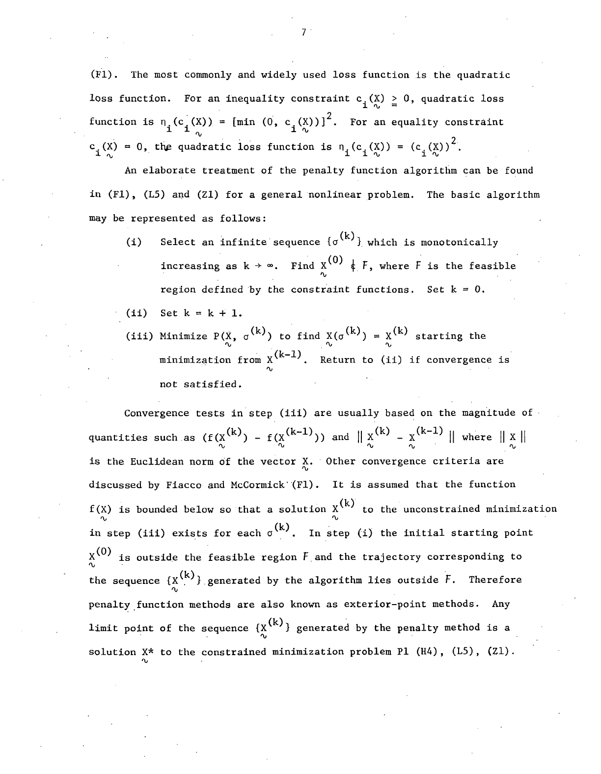
follows:

(k)

(i)

Select

an

infinite sequence

{a }

which

is

monotonically

increasing

as k

-»•

°°.

Find

X i F>

where

F is the

feasible

a.

region defined

by the

constraint functions.

Set k = 0.

(ii)

Set k = k + 1.

(iii)

Minimize

P(X,

a^')

to

find

X(a^)

= X^'

starting

the

f\j

r

O 'Y*

(k-1)

minimization from

X .

Return

to

(ii)

if

convergence

is

not

satisfied.

Convergence tests

in

step

(iii)

are

usually based

on the

magnitude

of

quantities such

as

(f(X

(k)

)

-

f(X

(k

~

1}

))

and ||

X

(k)

-

X

(k

~

1)

||

where

|| X ||

is

the

Euclidean norm

of the

vector

X.

Other convergence criteria

are

discussed

by

Fiacco

and

McCormick'(Fl).

It is

assumed

that

the

function

(k)

f(X)

is

bounded below

so

that

a

solution

X to the

unconstrained minimization

*\, 'Xf

(k)

in

step

(iii)

exists

for

each

a . In

step

(i) the

initial starting point

X^

' is

outside

the

feasible region

F and the

trajectory corresponding

to

<\j

the

sequence

{X . }

generated

by the

algorithm lies outside

F.

Therefore

•v

penalty function methods

are

also

known

as

exterior-point methods.

Any

(k)

limit

point

of the

sequence

{X }

generated

by the

penalty method

is a

solution

X* to the

constrained minimization problem

PI

(H4), (L5), (Zl).

The

penalty function technique might

be

regarded

as a

"primal"

approach

to

implicitly account

for the

constraints, although

its

connections with

duality

are

known

(Fl), (L5), (Zl).

The

approximation

of the

constrained

problem

by the

unconstrained penalty problem becomes more

and

more exact

as

the

control parameter

a -> °°.

However considerable computational difficulties

are

experienced with

the

traditional penalty function algorithm

as o -> °°.

These difficulties

are

delineated

in

detail

in

references (L3), (L5), (M5),

(Rll).

The

computational difficulties arise from P(X,

a)

forming

an

increasingly

'v

steep-sided

valley

as the

control parameter

is

increased

to

allow

the

unconstrained solutions

to

approach

the

constrained solution

to Pi

from

outside

the

active constraints.

In

particular,

the

Hessian

matrix

of the

penalty

function

[1]

becomes extremely ill-conditioned

as a

increases.

This leads

to

numerical

instabilities during unconstrained minimizations

of

the

penalty function

and

slow

convergence

of the

algorithm.

Attempts

to

overcome these computational difficulties have resulted

in

several modifications (Fl), (F2), (L3)

to the

penalty function technique.

Hestenes (H2)

and

Powell

(P3),

at

about

the

same time, independently

proposed

modifications that resulted

in a new

method related

to the

penalty

function

technique.

In

this

new

-method

penalty terms

are

added

to the

Lagrangian associated with

the

original

constrained problem. Hestenes (H2)

termed

this

the

"Multiplier Method".

It has

become

known

as the

Augmented

Lagrangian Penalty Function Technique

in

subsequent discussions. This

method

alleviated some

of the

computational difficulties associated with

the

traditional penalty function technique (F8)

and

achieved

better

convergence properties than

the

method

of

penalty functions (HA).

This

method

is

reviewed briefly

in

Chapter

3.

2.2

Lagrangian

Primal-Dual

Method

The

Lagrangian primal-dual method transforms

a

constrained convex

programming

problem into

a

sequence

of

unconstrained minimizations

of the

classical Lagrangian associated with

the

constrained

minimization

problem.

The

constrained problem

PI

becomes

a

convex programming problem when

the

objective

function f(X)

is

convex

and the

constraints c.(X)

i = 1, 2,

...,

m

a.

la.

are

concave.

The

concept

of the

primal-dual method

was

first implemented

by

Arrow,

et al.

(Al)

in the

differential gradient scheme

for

approaching

the

saddle-point

of the

Lagrangian L(X,

X)

associated with

a

convex program.

Oi "(j

The

Lagrangian associated with

the

convex problem

PI may be

represented

as

m _

L(X,

X) = f (X) - E X.

c.(X),

X £ L %• E

n

, X e E . [2]

'X*

*\j fYi • i 1 •*- 'Xf 'Xl *\» •

-v

1=

j_

m

where

E is the

nonnegative orthant

of

m-dimensional

Euclidean

space

E

m

and

the

vector

X e E, is

called

a

vector

of

multipliers.

Suppose

that

a

point

X*

satisfies

the

constraints

of the

convex program

PI and the

problem functions

are of

class

C . If

there exists

a

vector

X*

such that

X*

> 0, X.*

c.(X*)

= 0 V i and

VL(X*,

X*) =0, [3]

— i i a. a, <\, i\,

then

X* is a

global solution

to the

convex program

PI. The

vector

X* is

a.

^

said

to be the

vector

of

Lagrange multipliers associated with

X*. If the

.

- a.

gradients

of the

active constraints

at X* are

linearly independent, then

X*

<\i

• a.

is

a

regular point

of the

feasible region

F and

there exists

a

vector

of

Lagrange multipliers

X*

satisfying [3].

The

conditions

in [3] are

called

a.

the

Kuhn-Tucker first-order necessary conditions

for X* to be a

solution

to

1Q

PI and for the

convex program

PI,

these

are

also sufficient conditions

for

X* to be a

global solution.

For a

nondifferentiable convex problem

PI let

<\j

n

m

there

exist

an X* e E and a X* e E.

such

that

the

pair (X*,

X*) is the

^ >\j ^ ^

saddle-point

of the

Lagrangian L(X,

X)

-associated

with

the

convex program

* . 'x. a.- .

PI,

i.e., L(X*,

X) <

L(X*,

X*) <

L(X, X*).

Then

X* is the

global solution

r\,

r\j ~ ^ ^ —

1>

r

l>

. r\,

to

the

convex program

PI and X* is the

vector

of

Lagrange multipliers

a.

associated

with

X*.

oj

The

differential

gradient scheme

of

Arrow,

et al.

(Al)

for a

convex

program

may be

viewed

as a

small-step

primal-dual

method

where estimates

of

X* and X* are

modified

at

each iteration

to

exploit

the

saddle-point

'Xi

Oi

nature

of

L(X,

X)

near (X*, X*). This structure

of the

method

is

revealed

f\,

<\, f\j ^ • .

by

the

system

of

difference equations formulated

by

Uzawa (Al)

to

represent

the

differential gradient method. Davis (Dl) represents

the

iterations

in

this method

as

B-LCX,

x

(k)

)

r\,

1 1 <Vi 'Vi 'Vi

(k+1)

_ (k) -1 (k) (k)

X

= mm ID, X - a. o

VXL(.X

, X J

where

a and a are

scalars

representing step-size, VL(X,

X) is the

gradient

X 2. . <\( <\, o>

of

L(X,

X)

with respect

to X,

VXL(X,

X) is the

gradient

of

L(X,

X)

with

'X-

% f\j

'X/X< •'X;

'X. 'X/ 'Xi

respect

to X and B and B are

positive definite matrices

of

order

n and

r\j

1 i

(0)

m

respectively.

The

algorithm

may be

started

at any X

v

' e F and X e E,.

'X, »\» "*"

As

the

constrained problem

in the

above method

is

convex,

the

Lagrangian L(X,

X) is

also convex with respect

to X. The

iterations

on

'x/

a. <\/

(k)

X ,

therefore,

are

descent iterations

on

L(X,

X) and

update

of

multipliers

r\j 'Xl "Xl

11

X

may be

viewed

as

ascent iterations

on

L(X,

X). The X

update

may

O.

i\, r\, %

also

be

regarded

as

approximate solutions

to the

associated dual problem

(k)

at

X^ . The

dual associated

with

PI is .

<\,

m

Dl":

Maximize

l/(X)

over

all X e E

a.

^>

+

l/(X)

=

infimum L(X,

X) , X e L .

'Xi

'V 'Vi *X»

The

Lagrangian L(X,

X) is

minimized over

X e L for a

sequence

of

multiplier

"(j

Oi TJ

(k)

vectors

X and the

algorithm

is a

primal-dual method. Methods that

are

a.

similar

in

concept

to

this algorithm

are

described

by

Powell (PA)

,

Bertsekas

(B4)

, and

Lasden (LI)

.

The

algorithms based

on

Lagrangian primal-dual method

are not

susceptible

to

numerical

instabilities

such

as

those

discussed

in

connection

with

the

penalty method. Primal-dual methods

are

based

on the

viewpoint

that

the

Lagrange multipliers

X* are

also fundamental

unknowns

associated with

a

%

constrained problem. This

is due to the

reason

that

Lagrange multipliers

measure sensitivities

and

often have meaningful interpretations

as

prices

associated with constraint resources (H4)

,

(L5). Useful duality results

for

convex programs have been presented

by

Luenberger (L5)

and

Zangwill (Zl)

.

Various formulations

of the

duality theory

for

nonlinear convex programs

using

the

classical

Lagrangian have been reworked

and

extended

by

Geoffrion

(Gl)

so as to

facilitate, more readily, computational

and

theoretical

applications.

Methods based

on the

classical

Lagrangian

for

solving

a

constrained

problem

PI

have been reviewed

by

Lootsma (L3)

.

The

Lagrangian primal-dual method

is

known

to

have serious disadvantages

(R3)

,

(R6)

. The

most restrictive

one is

that

the

constrained problem must

12

be

convex

In

order

for the

dual

problem

to be

well

defined

and X

iterations

<\>

to

be

meaningful.

In

general

inf

(PI)

> sup

(Dl)

and the

equality holds

good

only

for the

convex problem

PI. For

nonconvex problems only

the

inequality

hcvlds

in the

above relationship

and in

such cases

a

duality

gap

is

said

to

exist.

For

nonconvex problems Everett (E2) introduced

a

primal

dual

method called generalized Lagrange multiplier method. This

and

other

associated methods

are

summarized

by

Lootsma (L3). Even though Everett (E2)

suggested

some methods

of

handling

the

duality gap,

the

method

has

been

found

to be

useful only

for

certain

nonlinear

problems with special structure.

The

method

is of

importance

in the

decompoisition

of

large-scale problems

with separable functions.

In

such cases minimization

of the

Lagrangian

can .

be

carried

out

efficiently

due to the

special structure

of the

constrained

problem

(E2), (LI), (L5).

For

a

convex program,

if X* is the

optimal solution

to the

constrained

"u

problem

with corresponding Lagrange multiplier vector

X*,

then

X* is the

>\j

<\,

unconstrained minimizer

of

L(X, X*). However,

if X* is a

local solution

to

a.

a. . ^

a

nonconvex program with corresponding Lagrange multiplier vector

X*,

then

^

X* may not be the

unconstrained local minimizer

of

L(X,

X*) and

L(X,

X*) may

^ r\j ^ ^ Oi

even

have negative second derivatives

at X* in

certain directions normal

Oi

to

the

feasible manifold

F

(R3). Since curvature

at a

point

is

determined

by

the

second partial derivatives, attempts were made

to

make

the

Lagrangian

associated with nonconvex programs

a

convex function

by

adding quadratic

penalty

terms

to it.

This concept

was

first suggested

by

Arrow

and

Solow (Al)

in

connection with

the

solution

of a

nonconvex equality constrained problem

using

the

differential gradient method. Arrow

and

Solow augmented

the

classical Lagrangian with quadratic penalty terms

and

this

'elegant idea

13

made

the new

augmented Lagrangian locally convex. This idea

was

independently

reconsidered

in an

entirely different algorithmic context

for

equality

constrained problems

by

Hestenes (H2),

Powell

(P3)

and

Haarhoff

and

Buys (Hi).

The

algorithms

that

resulted from these efforts belong

to the

Augmented

Lagrangian Penalty Function Technique which

is

reviewed

in

Section

3.

14

III. AUGMENTED LAGRANGIAN PENALTY FUNCTION TECHNIQUE

3.1

Introduction

The

ALA'G

penalty function technique

may be

reviewed from

two

entirely

different

points

of

view.

The

first view-point

is

that

the

methods that

belong

to

this technique modify

the

Lagrangian associated with

a

nonconvex

or

a

weakly

convex constrained problem

to

have

a

local convexity property.

This

is

because

the

characterization

of

solution

to a

constrained problem

in

terms

of a

saddle-point

of the

Lagrangian depends heavily

on

convexity

properties

of the

underlying problem.

The

local saddle-point property

is

obtained

by the

presence

of a

convexifying parameter

in the

Lagrangian

which

makes

the

associated

Hessian

positive definite

for

large enough,

but

•finite,

values

of the

parameter.

Following

this idea

of

local

convexification

many

different modifications

of the

classical

Lagrangian have been proposed

to

close

the

duality

gap in

nonconvex programming (Al), (A2), (M2).

The

second viewpoint

is to

consider

the

technique

and the

quadratic

penalty

function method

within

a

common generalized penalty function frame-

work.

The

approach here

is to

circumvent instabilities associated with

the

classical

penalty function method

by

adding penalty terms

to the

Lagrangian

function.

The

advantages

of

using

a

first-order penalty furnction have

been

listed

by

Lootsma (L3)

and

McCormick (M5)

.

Therefore methods that

augment

the

Lagrangian with quadratic penalty terms

are

considered

in

detail.

The

development

of the

ALAG penalty function technique

is

traced from

the

second

viewpoint.

15

3.2

Review

of the

Technique

for

Equality Constrained Problem

3.2.1 Equality Constrained Problem

The

equality constrained problem

P2 may be

represented

as

follows:

•

P2:

Minimize f(X)

^

Subject

to

c.(X)

=0 i = 1, 2,

...,

m m < n

1

^ ~ • '

(2)

f(X)

and

c.(X)

i = 1, 2,

...,

m are

real-valued functions

of

class

C

defined

on a

nonempty open

set L SL. E . The

Lagrangian associated with

P2

is

m

L(X,

X) =

f(X)

- Z X, c

(X),

X e

E

m

..

[4]

l

\t

*\j

f

\j i 11 f\j f\.

±=1

The

gradient

and

Hessian

of

this

Lagrangian

with respect

to X are

VL(X,

X)

2

and

V

L(X,

X)

respectively.

*\/

f^j

Let

X* be an

optimal solution

to P2 and the

problem functions f(X)

(2)

and

c.(X),

i = 1, 2,

...,

m be of

class

C in an

open neighborhood

of X*.

The

following

are

assumed

to

hold

good

at X*.

(i) The

point

X* is a

regular point

of the

feasible

set

"u

F

= {X:

c.(X)

= 0 i = 1, 2,

...,

m, X e L S E

n

}

Let

N* =

N(X*)

be the nxm

matrix [Vc,, Vc

0

, ...,

Vc ].

r\j

i\j J. >\, Z ^ m

The

regularity

of the

feasible

set at X* is

satisfied when

N* is of

full

rank.

(ii) There exists

an

unique Lagrange multiplier vector

X*

such

that

the

following first-order necessary conditions

for

local optimality

at X* are

satisfied.

X*

e E

m

,

c.(X*)

= 0 Vi and

VL(X*.

X*) = 0. . [5]

f

\j

1 'V;

/

\J *X> *\>

16

(iii)

The

second-order

necessary

conditions

for

local

optimality

at

X* are

that

in

addition

to [5]

^

Y

T

V

2

L(X*,

X*) Y > 0 . V Y e V^ E" [6]

^ 'Xi % Oj — ^

V

= {Y: Y

T

Vc. = 0 Vi}

>\>

"u O, 1

(iv)

The

second-order sufficient conditions

for X* to be an

isolated

"c

local minimum

are

that

in

addition

to [5]

Y

T

V

2

L(X*,

X*) Y > 0 V

nonzero

Y e V [7]

^ O> "\j <\, ^ •

(v)

Strict complementarity holds

at X*,

i.e.

, X.* ^ 0 Vi

it 1-

3.2.2

Powell

-

Hestenes Augmented Penalty Function

Powell

(P3) suggested

the

following penalty function

to

solve

P2.

,

m

2

<Kx,

e, s) =

f(x)

+± z

o.(c.(x)

- e.)

*\i

<\i r\j 2. -I 1 1 O> !

=

f(X)

+ \

(c(X)

-

6)

T

S (c(X)

- 6) [8]

where

9 e E

m

,

C(X)

is a

vector

of

constraint functions

c . (X) i = 1, 2,

...,

m

o>

'Vi 'v • ' i *\<

and

S is a

diagonal matrix

of

order

m

with,

diagonal elements

a. > 0. Let

a e E be a

vector with

a. as

components. While

the

classical penalty

/\,

"*•*"

i

function

for P2

contains

at

most

m

control parameters,

the

above function

depends

on 2m

parameters which

are the

components

of 6 and a. The

main

f\j

i\,

difference between

classical

quadratic penalty function

and [8] is the

introduction

of

parameters

9. In [8]

quadratic penalty terms have been

<Vi

added

to the

Lagrangian associated with

P2.

The

augmented penalty function

(j>

is

used

in the

algorithm

as

follows.

17

Algorithm

Al:

(i)

Select 9

(1)

=0.,

k = 0,

S

(1)

= I and

X

(0)

i F.

o> >\j

(ii)

k = k + 1

(iii)

Minimize

<J>(X,

9

(k)

,

S

(k)

)

to

find

=

X(6 , S )

starting

the

unconstrained

*\i

^

minimization

from

X . .

>\,

(k)

(iv)

If C(X ) is

converging sufficiently rapidly

to

zero then

e

(k+l?

=

6

(k)

'Vl

^

=

s

(k)

and

return

to

otherwise

(i/io)

e

(k)

^

1Q

g

(k)

and

return

to

•In

step

(ii)

<|>

is

minimized with respect

to X

without constraints

for

fixed

<v/

(k) (k)

values

of 6 and S and

this

is the

inner iteration

of the

algorithm.

^

(k) (k)

Step

(iii)

is the

outer iteration

in

which

6 and S are

changed

to

%

(k)

force

constraint satisfaction

and

cause

the

sequence

of

solutions

{X }

^

to

converge

to X* at a

reasonably fast rate.

^

The

scheme

for

adjusting

0

parameters

in the

outer iteration

is

(k)

based

on the

observation

that

if

X

vr

"'

is the

minimizer

of

<j>(X,

9

V

~' , S

*v/

a. ^

(k)

in

the

inner

iteration, then

X is

also

a

solution

of the

problem

Minimize

f(X)

X e L <= E

n

Subject

to

C(X)

=

In

order

to

solve

the

equality constrained problem

P2 it is

sufficient

to

find

6

(k)

and

S

(k)

such

that

X

(k)

=

X(9

(k)

,

S

(k)

) solves

the

system

of

'Vi

f\, *\i 1*

nonlinear equations

18

C(X(6

(k)

,

S)) - 0. • [9]

The

above system

of

equations

is in

terms

of 2m

parameters

8 and a

i

(k) (k)

i = 1, 2, . . . , m. One

vector

of

parameters

0 or. a may be

fixed

and

[9]

then

is a*

system

of m

equations

in m

remaining parameters.

(k)

If

6 is

fixed, then

[8]

reduces

to a

basic penalty transformation.

f\j

Specifically when

0

parameters

are set to

zero,

$

becomes

the

classical

<\j

quadratic

penalty function.

In

such

a

case convergence

of the

sequence

(k)

{X } to X* is

ensured

by

letting

a.

-*•

°°, i = 1, 2 . . . , ra.

This leads

a-

'v i

to

numerical instabilities

and

slow convergence. Therefore

in

Powell's

(k) (k)

method

S is

held constant

and 0 is

changed

to

force constraint

<\,

satisfaction through iterative solution

of

[9].

Powell

(P2)

derived

a

(k) (k)

simple correction

for

adjusting

0

parameters when

S is

fixed

by

'V

•applying

generalized Newton iteration

to

solve

[9].

This correction

is

represented

as

(k)

'

(k)

(k) (k)

By

definition

X is the

unconstrained minimizer

of

<j>(X,

6 , S ).

Oj "\> O;

Therefore

V4>(X

(k)

,

0

(k)

,

S

(k)

)

= 0,

i.e.,

Vf(X

(k)

)

+ I

a.(C.(X

(k)

)

-

0.

(k)

)

VC.(X

(k)

)

= 0.

[11]

Continuity

of

C(X)

in the

neighborhood

of the

local minimizer

X* of P2

<X>

'Xi • 'Vi

(\r\ df-V

implies

that

the

matrix

N(X

V

') is of

full rank

for X

v

'

sufficiently close

/U\

to

X*.

When

X

v

' is in the

neighborhood

of X* and

when

X

v

'

->-

X* the

estimates

X

(k)

=-S

(k)

(C(X

(k)

)

-0)

[12]

i\,

19

exist

and

have

as

limit points

the

unique values

X* = S* 9*,

where

9* and S*

are the

parameters corresponding

to X*.

Hence

the

final value

of the

product

S 9, in the

limiting sense,

is a

constant

and may

considered

to be

independent

of S

when

S is

fixed

and 9 is

adjusted

to let 9

-»-

6*. Due to

• <\, "" <\,

this

reason, when

S is

increased

in

step (iii)

of

algorithm

Al to

improve

the

rate

of

convergence

of the

sequence

{max|c.(X

. • )|) to 0 and {X } to

,

i ^

X*, 6 is

decreased

to

keep

S 9 a

constant.

Convergence

of the

algorithm

is

measured using

the

sequence

{max|c.(X

)|),

Under

the

assumptions

in

3.2.1

and

when

the

Hessian matrix

of

<}>

is

positive

definite

at X*,

Powell

(P2) proved

that

the

rate

of

.convergence

is

linear

and

the

convergence ratio depends

on

I/a.

for a. > a

1

. The

threshold value

a' is a

large

but

finite positive real number. Therefore

by

choosing

S to

be

large

so

that

S is

close

to S',

where

S

1

=

a'I,

the

algorithm

can be

made

to

have linear convergence

at any

arbitrary rate. Superlinear convergence

is

achieved when

a. -> °°. In

Powell's

algorithm

the

rate

of

convergence

is

taken

to be

satisfactory when

the

maximum residual,

max|c.(X

)|, of the

system

of

equations

[9] is

reduced

by a

factor

of

four

on

each iteration.

The

reason

for

preferring

the

slower rate

of

convergence implied

by the use

of

factor four

is

that faster convergence tends

to

make

the

inner iterations

(k)

more difficult (P2).

When

the

sequence

{max|c.(X

)|)

either fails

to

converge

or

converges

to

zero

at too

slow

a

rate,

S is

increased

by a

factor

of

ten.

The

choice

of

factor

ten to

increase

S is

arbitrary.

Numerical evidence indicates

that

the

value

of a is

seldom required

to

2

be

greater than

10 to

ensure rapid convergence

(Rll).

The

Hessian matrix

of 4>

depends

on

both

9 and S. The

change

in

this

matrix

is

dominated

by the

increase

in S

(P2). This

is

another reason

20

for

using

a

factor

of ten to

increase

S

when

the

rate

of

convergence

is

slow

and

keeping

S

constant when rate

of

convergence

is

satisfactory.

If

S is

chosen

to be

large

in the

initial iteration, instead

of

gradually

increasing

S, the

Hessian

of

<|>

becomes ill-conditioned

and the

unconstrained

•

minimization

of

<J>

in the

inner iteration becomes very difficult

to

perform.

Further

for a

large

S, an

arbitrary starting point

X ' and

arbitrary values

'Vi

(k)

of

0

parameters,

the

sequence

(X } may not

converge

to X*.

Therefore

S

a, . • r\, <^

(k) (k)

is

increased

so as to

force

X

into

a

region

in

which

sequence

{X }

^ <\,

locally converges

to X*.

Once this region

is

reached,

S is

kept constant

(k)

and

6

parameters

are

adjusted

so as to let X

-»•

X*.

Further

the

gradual

<\,

<x, %

increase

of S is

designed

to

make

<f>

continuous

and

continuously

dif

ferentiable

with respect

to X for all

values

of the

parameters.

In

Powell's

algorithm

the

minimizations

in the

inner iteration

are not

beset

by

computational

difficulties associated with

the

basic penalty function transformations.

The

minimizations

are

well

scaled

and

progressively less computational

(k)

effort

is

required

as k

increases

and X

->•

X*.

1j "Vi

Hestenes (H2)

,

independently

of

Powell

and at

about

the

same time,

proposed

a

similar method

for

solving

P2 and he

called

it the

method

of

multipliers.

The

method

is

based

on the

observation

that

if X* is a

^

nonsingular minimum

of P2,

there exists

a

multiplier vector

X* and a

constant

Oj

a

such that

X*

affords

an

unconstrained local minimum

to the

function

T(X,

X*, S) =

f(X)

- X*

T

C(X)

+ 1/2

(C(X))

T

SC(X)

.

[13]

'V.'V.

O>'X<f\,'Vi

Of'X.'V'Xi

where

S = ol.

Conversely,

if

C(X*)

= 0 and X*

affords

a

minimum

to

[13],

^ 'Vi 'Vi

then

X*

affords

a

minimum

to P2. In the

method

of

multipliers

a

large

21

positive

constant

a is

suitably chosen

and is

held fast.

The

augmented

penalty function considered

is

T(X,.X,

S) =

f(X)

- X

T

C(X)

+ 1/2

(C(X))

T

SC(X) [14]

i

r r i

where

X e B and 8 is an

arbitrary compact subset

of E . The

function

in

/

v>

[14]

is

sequentially minimized

for

successive estimates

X of the

unique

a. .

Lagrange multiplier vector

X* at X*.

"Xi

^i

(k) (k)

The

unconstrained minimization

of

T(X,

X , S) for an

estimate

X

r\,

<\, %

(k) (k)

of

X* is the

inner iteration.

Let X = X(X , S) be an

unconstrained

^ -v i,

(k) (k)

minimizer

of

T(X,

X , S) . In the

outer iteration

the

estimate

X is

a.

a/ ^

(k)

updated

so as to

cause

X -> X*.

Hestenes suggested

the

following

formula

'V

O;

(k)

for

adjusting

the

multiplier vector

X

a.

where

S = o I, 0 < a <. a, a = yo and 0 < y < 1- The

relation

(k)

[15]

is

derived from

the

observation

that

X is a

local minimizer

of

-v

(k)

(k+1)

T(X,

X , S) and X is

chosen

so

that first order necessary conditions

^ <\, ^ .

(k)

are

satisfied

at X for P2.

Hestenes

(H2)

did not

analyze

the

convergence

of

the

method,

but

subsequently (H4) established that

the

method converges

linearly

and

superlinear convergence

may be

achieved when

a

-»•

°°. In

practical

applications very fast linear convergence occurs

for a

large

but

finite value

of o.

Convergence

is

induced

by not

only

a

large value

of

a but

also

by

multiplier iteration [15] (F8)

.

In

Powell's

method when

S is

fixed

and 6

parameters

are

adjusted

to

'V

(k)

let

X

->-

X*, the

unique Lagrange multiplier vector

X* = S 6*,

where

6*

22

corresponds

to the

vector

of

parameters

at X*.

This implies

that

a

'Xi

connection

can be

established between

the

augmented function

<f>

in [8] and

T in

[14]

using

the

relationship

i

V

i =

1> 2>

'"'

m

'

From

[8], [14]

and

[16],

1

m

2

<KX,

0, S) =

T(X,

X, S) +± Z \

.la.. [17].

r\j

<\, >\j f\j L

._•]

J- 1

The

difference between

<f>

and T is

independent

of X. If

X(6,

S) and

X(X,

S)

'X-

<V; O. 'X/ O>

are

unconstrained

minimizers

of

<j>

and T

respectively

for any S and if 6 and

a.

X

are

[16],

then

X(6,

S) =

X(X,

S).

Therefore

the

iterative

<\,

fx, Oi *\J i\,

-methods

suggested

by

Powell

and

Hestenes

for

changing

9 and X

parameters

'Vi

'Xi

are the

same.

In

view

of the

equivalence relationship

[17]

between

cf>

and T, the

numerical algorithm

Al is

discussed

in

terms

of the

augmented penalty

function

T. - In the

outer iteration adjustment

of X

parameters using

[15]

%

is

considered, assuming

that

6 and X are

[16].

The

algorithm

f\, 'Xi

Al is

discussed

and

analyzed using

X

parameters

to

emphasize

the

primal-dual

<\j

(k)

nature

of the

method which iterates with

an

approximation

X to the

'V,

(k)

Lagrange multipliers

X* in

such

a way as to

make

X •*• \*.

'Xi

^

The

algorithm

Al is now

modified

and

denoted

as the

Powell-Hestenes

augmented

penalty function algorithm

A2. The

convergence

of the

algorithm

is

measured

in

terms

of B =

max|c.(X)|.

23

Algorithm

A2:

(i)

Select

X

(1)

=

X

(0)

, S

(1)

=

S

(0)

,

k = 0,

arbitrary starting

point

X

(0)

and

B

(1)

= B_

where

B

0

>

max!c.(X

(0)

)I.

'v.

0 0 = . ' i

<\,

'

i

(ii)

k = k + 1

(iii)

Minimize

T(X,

X

(k)

, S

(k)

)

to

find

X

(k)

=

X(X

(k)

,

S

(k)

)

(k-1)

starting

the

unconstrained minimization from

X

a.

(iv) Find

V = {i:

|c

±

(X

(k)

)|

>

B

(k)

/4}.

If

max|c

(X

(k)

)|

>

B

(k)

,

set

B

(k+1)

-

B

(k)

.

Go to

(vii).

•

1 *\; ^

1

(v)

B

(k+1)

=

max|c

i

(X

(k)

)|.

If

B

(k+1)

< E

stop.

The E is a

i

specified

tolerance

for B.

(vi)

If

B

(k+1

>

<

B

(k

V4

or

X

(k)

= X

0

^

*\»

^

set

X -

A<

k

>

-

S

(k)

C(X

(k)

)

,

go to

(ii).

(vii)

Set

X

(k+1

>

=

X

(k)

Ck+11

Ck} ^

yixi^j.y

i f*.

VR./ TT'•

TI

o.

- 10 o Vi e V,

i i

go

to

(ii).

When second order sufficiency conditions hold good

at X* for P2,

there exists

Oi

a a

1

> 0

such

that

for o. > a

1

Vi, the

Hessian matrix

of

both

(j>(X,

6*, S)

and

T(X,

X*, S) at X* is

positive definite

and X* is a

strong local minimum

of

<j.(X,

6*, S) and

T(X,

X*, S)

(B2), (B7),

(F8),

(H2)

. It

should

be

noted

'V

^ 'V/

that

the

local convexity

of

<j>(X,

9*, S) and

T(X,

X*, S)

near

X* is

established

without

any

assumptions about

the

convexity

of

problem

P2. The aim of the

(k) (k)

algorithm

A2 is to

.keep

S

constant

and

adjust

X so as to

cause

X -*• X*.

f\j *V *X»

24

Therefore

in

subsequent discussions

it is

assumed

that

a. > a

1

Vi

have

been

chosen

and

held fast

so

that

(j>

and T are

locally convex.

Due to

this reason

the

explicit dependence

of X on S is

dropped

and

X(X,

S) is

represented

as

f\j

^ 'V

X(X).

%

<\,

•

Haarhoff

and

Buys (HI) proposed

a

numerical algorithm very similar

to

the

Powell-Hestenes method. They were motivated

by the

following observations

about

the

traditional quadratic penalty function approach

to

solve

P2. Let

the

quadratic penalty

function

for P2 be

m

2

P(X,

a) =

f(X)

+ a Z

(c.(X))

, a > 0.

Let

X(a)

be an

unconstrained

minimizer

of

P(X,

a) for a

large value

of

'o r\j

control

parameter

a and X* be a

local minimizer

of P2. The

gradient

of

<v

P(X,

a) is

zero

at

X(a)

but the

gradient

at X* is

Vf(X*).

Therefore,

in the

'Y/

f\, . 'V . i\, O.

usual case when

Vf(X*)

is

nonzero, X(a)

and X*

have

to be

different.

Let X

'V

^ ^ ^ ^

be

a

solution

to the

under-determined system

of

equations C(X)

=0. At X

a. <\j a.

the

gradient

of

P(X,

a) is

Vf(X) which

is

generally,

not

zero. Therefore

X

>\j

Oi "Xi ^J

and

X(a)

are

different

and for any

finite value

of a,

X(o)

is

neither

a

"u

. ^

solution

to P2 nor

satisfies C(X)

= 0.

Usually X(o) tends

to X*

when

a -> °°

a/ 'v/ *v> a.

(L5), (Zl). From these observations Haarhoff

and

Buys added

a

linear

combination

of

constraints

to

P(X,

a) to

obtain

a.

T(X,

X, S) - f (X) - A

T

C(X)

+ ^

(C(X))

T

SC(X),

S =• ol

"

where

X e E and o > 0.

This function achieved their objective, i.e.,

a.

balanced

the

gradient

of

f(X)

in the

vicinity

of the

minimum

by a

linear

^

combination

of

gradients

of

constraint functions C(X).

r\, <\j

25

The

augmented penalty function proposed

by

Haarhoff

and

Buys

is .

identical

to the

Powell-Hestenes

augmented penalty function

for P2.

However

.

the

numerical algorithm

of

Haarhoff

and

Buys

has

some distinct features.

They noted

that

the

multiplier updates

[15]

are

valid only

when

the

function

(k)

T(X,

X , S) is

minimized exactly

for

each

X and

that

it is

better

to

*V *\j 'X*

(k)

terminate

the

inner iterations when

a

better value

of

T(X,

X , S) is

obtained. They suggested that

the

multipliers.in

the

outer iteration

be

obtained

from

the

first order necessary condition.

Vf(X

(k)

)

=

N(X

(k)

)

X, X e E

m

. .

[18]

The

condition

[18]

represents

an

over-determined system

of n

equations

in m

(k)

parameters.

Taking

the

scalar

product

of

[18]

with each VC.(X

), the

<\,

i a,

following

system

of

equations

is

obtained.

N

T

(X

(k)

)

Vf(X

(k)

)

=

N

T

(X

(k)

) N(X

(k)

)

X, X e E

m

.

[19]

^ <\, ^ ^ a. a. a.

The

expression

in

[19]

represents

a

system

of m

equations

in m

parameters

X

that

may

easily

be

solved

for X.

This,

in

effect,

is a

least squares'

'V

^

solution

to

[18].

The

vector

of

multipliers

X is an

estimate

of the

unique

a/

Lagrange multiplier vector

X* at X* and X

tends

to A*.

% >\j -V ^

Haarhoff

and

Buys were more concerned with computational considerations

than

with convergence

or

duality aspects

of the

algorithm.

They

suggested

that

the

problem functions

be

scaled

so

that

the

gradients

are of the

same

magnitude

and o. be on the

order

of

ten.

In

this algorithm

a. i = 1, 2,

...,

m

are

kept constant

and in the

inner iteration

the

variable metric method

of

26

fir)

Davidon-Fletcher-Powell (DFP)

is

used

to

minimize

T(X,

X • ., S). The

^ ^

2-1

approximation

to [V T] is

updated using

the DFP

update formula

(Mil).

A

restoration

step

is

included

in the

inner

iteration

and in

this step

T

is

minimized without using derivatives

in a

direction

that

leads

to the

satisfaction

of

linearized constraints. Other numerical aspects

of the

algorithm,

such

as the

various stopping criteria

for

inner

and

outer

2

-1

iterations

and

updating

the

approximation

to

inverse Hessian

[V T] are

discussed

in

reference (HI).

The

elegant idea

of

local convexification

of the

Lagrangian

was

first

introduced

by

Arrow

and

Solow (Al). They suggested addition

of

quadratic

penalty

terms

to the

classical Lagrangian

to

arrive

at a

modified Lagrangian

that

was

locally convex. They were motivated

by

adaptation

of the

differential gradient scheme, developed

by

Arrow,

et al.

(Al)

for

approaching

saddle points

of

convex programs,

to

nonconvex programs. Their

differential

gradient method

is a

small step-size algorithm while those

of

Hestenes, Powell

and

Haarhoff

and

Buys

are

large step-size methods.

In the

above contributions

to the

augmented penalty function technique

duality

concepts were

not

employed. Primal-dual interpretation

of the

technique

was

analyzed

by

Buys (B7), Luenberger (L5), Rockafellar (R12)

and

Bertsekas (B2), (B3).

A

detailed review

of the

duality results

may

be

found

in

reference (F8).

The

duality results

are

summarized briefly

in the

next section.

3.3

Review

of the

Technique

for a

Constrained Problem with Equalities

and

Inequalities

3.3.1 Constrained Problem

The

problem

P3

with equality

and

inequality constraints

is

represented

as

27

P3:

Minimize

f(X),

'X e L £: E"

Subject

to

c.(X)

= 0 i = 1, 2,

...,

k

i

%

c.(X)

> 0 i =

k+1, ...,

m, 0 < k < n.

i <\, - = =

The

real valued functions

f(X)

and

c.(X)

Vi are

defined

on a

nonempty open

a,

x

•>

set

L£ E . Let X* be a

local optimal solution

to P3. The

problem functions

(2)

are

of

class

C on L and

specifically

in an

open neighborhood

of X*. The

Lagrangian associated with

P3 is

rp

m

L(X,

A) =

f(X)

- A

C(X),

A e E , X e L £; E .

[20]

The

following conditions

are

assumed

to

hold good

at X*

(Fl), (M13).

(1) X* is a

regular point

of the

feasible region

a.

F

= (X: C. (X) = 0, 1 < i < k and

C.(X)

> 0, k < i < m}

Let

E = {i: 1 < i < k}

I = {i:

C.(X*)

=0, k < i < m}. The X* is a

regular point

i

<\,

• — ^

of

F

when

{VC.(X*)}

i e E £ I is a

linearly independent

set,

i\,

1 <\,

(2)

There exists

an

unique Lagrange multiplier vector

A* e E

such

that

the

Kuhn-Tucker

conditions

are

satisfied

at

(X*,

A*)

C.(X*)

= 0 i e E

C.(X*)

> 0 A.* > 0, A.*

C.(X*)

=0 i £ e

[21]

1 *\y — '1 — 3. 'Xj

VL(X*,

A*) = 0

'X/

f\j r\j

These

are

first-order necessary conditions

for

local optimality

at

X* and (X* A*) e E°

satisfying

[21]

is

termed

a

Kuhn-

'X,

'X. 'X.

Tucker point.

28

(3)

Second-order necessary conditions

for

local optimality

of X*

a.

are

that

in

addition

to

[21]

Y

T

V

2

L(X*.

A*) Y > 0 VY e /*

SrE

n

.

[22]

~

where

V*

= {Y: Y

T

VC.(X*)

= 0, i e E S I* and

'v

'v ^, i <\,

Y

T

VC.(X*)

> 0, i e

I-I*},

-

I is the

index

set of

active inequalities,

I* is the

index

set

of

strongly active inequalities

and I - I* is the

index

set of

weakley active constraints. However

the

following weaker

second-order necessary condition

is

usually assumed instead

of

[22] (Fl),

(Mil).

Y

T

V

2

L(X*,

A*) Y > 0 V Y e V£. E

n

[23]

%

'v a/ - %

V

= {Y: Y

T

VC.

(X*)

= 0, i e E

<~l}.

i\j

i\, r\j 1 'X,

(4)

Strict complementarity holds

at

(X*,

A*)

when

a. 'x.

A.*

j 0 for

each

1 < i < m for

which

C.(X*)

= 0.

[24]

1 = 1 'V,

A

weaker

form

of

[24]

is

A.*

> 0 and

C.(X*)

= 0, i e I.

[25]

i i -x,

(5)

Second-order sufficient conditions

for X* to be an

isolated

>\,

local minimum

are

that

in

addition

to

[21]

and

[23]

Y

T

V

2

(X*,

A*) Y > 0 V

nonzero

Ye/*. [26]

29

However

the

condition

[26]

is

usually replaced

by the

verifiable

condition

(Mil),

.Y

T

V

2

L(X*,

X*) Y > 0 V

nonzero

Y e V.

[27]

3.3.2 Powell

-

Hestenes

-

Rockafellar Penalty Function

The

augmented Lagrangian penalty function

for P3 is

obtained

by

combining

the

Powell-Hestenes penalty function

T and the

Rockafellar penalty

function

T. The

combined function

may be

represented

as

T

DU1

,(X,

X, a) =

f(X)

- E [X,

C.(X)

- ^ ° •

C,

2

(X)]

+

ieE

--•*,'--•*.

[28]

\ E [a (C (X) -)

2

- X

2

/a ]

2

where

X. X.

(C.(X)

- —) = min

[(C.CX)

- —), 0]

i o, a. la. a.

,-m

c

m

a e c,, , X e E .

"~"

In

[28],

the

factor

X./a.

represents

a

penalizing threshold

for the ith

inequality constraint.

The

multipliers

X. Vi are

unconstrained

and

this

is

an

useful property

of the

augmented penalty function

T .

Further

the

r

HK

function

T

possesses

a

number

of

strong properties

not

exhibited

by the

PHR

classical Lagrangian

L(X,

X). The

following properties

of T

D

make

it

r.

f\j r UK

ideal

for use in. a

primal-dual algorithm

for

solving

P3.

Let

M(X)

be the

index

set of the

inequalities

that

contribute

to

the

quadratic penalty term

in T for an

estimate,

X, of the

Lagrange

Jr

UK f\j

30

multiplier

vector

A*.

'V

•-M(X)

= {i: i i E,

C

±

(X)

< A

/oi}. [29]

Equivalently,,

M(A)

= {i: ± \. E, A. - a.

C.(X)

> 0}. .

[30]

•\»

1 1 1

*\/

At

the

local optimum (X*,

A*) of P3,

M(A*)

is the

index set,

I*, of the

strongly active inequalities.

By the

strict

complementarity assumption,

I = I* and

therefore M(A*) represents

the

active inequality constraints

at

the

local

optimum

(X*, A*). Further

the set

EUM(A)

represents

the

*\»

*\t ^

inactive inequality constraints

at the

intermediate approximation

(X, A) to

the

solution (X*, A*).

Let L = E

LTM(A).

Then,

'v <x, a.

L = {i: i i E.

C.(X)

>

A./a

}.

[31]

1^ — 11

Equivalently,

L

= {i: i i E, A. - a.

C.(X)

> 0}.

[32]

•vl

1 1

<X/

—

Using

the

above results

the

augmented penalty function

T may be

FHK.

represented

as

follows.

r_

UD

(X, A, a) =

f(X)

- E (A.

-~a.

C.(X))

C.(X)

FHK

'V-'X.'X.

-X.

j,T7

vr/->\

X

/ll'X,

1

ieE

M(A)

[33]

1

v

-. 2,

- Z A.

/a..

2 .

T

i i

31

The

representation

of T in

[33]

clearly illustrates

that

it is

obtained

rHK

by

combining

the

Powell-Hestenes penalty function

T and the

Rockafellar

penalty

function

T.

Mangasarian

(M2)

associated

a

wide class

of

Lagrangians with

the

nonconvex program

P3. The

unconstrained stationary points

and

local saddle-

points

of

each Lagrangian were shown

to be

Kuhn-Tucker

points

or

local

or

global

solutions

of P3

(M2),

The

Lagrangians considered

by

Mangasarian

(M2)

were

twice differentiable globally.

The

augmented penalty

function

T

belongs

to the

general

class

of

Lagrangians investigated

by

rnK

Mangasarian

(M2)

.

However

the

penalty function

T^.,-,

is

twice continuously

rHK

differentiable

in X

except

at

points where

X. - a.

c.(X)

=0, i e

M(X).

ft 1 1 1

*"\j

f\j

By

the

strict complementarity condition,

X. - a.

c.(X*)

^ 0 for i e

H(X*~)

,

1 X 1 'X/ 'V •

i.e.,

i e I.

Therfore

T is

twice continuously differentiable

in an

open

rHK

neighborhood

about

(X*, X*).

Oj Oj

Mangasarian

(M2)

established

the

properties

of the

general class

of

Lagrangians

for P3. As T is a

member

of

this class

of

Lagrangians,

PHR

the

following properties hold

good

for

T_.._.

(M2)

.

.These properties

of T

rnK rHK

also were established

by

Rockafellar

(R6).

For a e E ,

(X*,

X*) is a

f

\j * * *\;

f

\j

Kuhn-Tucker point

of P3 if and

only

if it is a

stationary point

of T „.

rHK

2

For

large

but

finite

a., V T_, is

positive definite

(M2), (A3)

and

1 rHK

T

(X*,

X, o) < T

(X*,

X*, a) < T (X, X*, a)

rnK f\j r\j r\j —

rni\.

r\j *\, ^v» —

rntv

r\j f\,

.V

X e E , X e A

where

A is

some open neighborhood

of X*.

Conversely,

if

(X*,

X*) is a

saddle-point satisfying

[34],

then

X* is a

solution

of P3

for X e A.

[34]

32

A

duality theory

in

terms

of

extended

Lagrangians

was

presented

by

Mangasarian

(M2).

The' augmented dual problem

may be

represented

as

D3:

Maximize

g(X,

a).

a.

g(X,

a) = inf T (X, X, a)

f\j

f\j V /

tllx

i\f r\j

[35]

The

augmented dual function

g(X,

a) is

concave

in (X, a) and is

strictly

nondecreasing

in a. If the

point (X*,.

X*)

satisfies

the

optimality conditions

and

if a is

sufficiently large, then

(X*,

X*) is an

isolated local maximum

of

D3.

Conversely,

if

(X*,

X*) is a

global

or

local solution

of D3,

then

the

optimality conditions

for P3 are

satisfied

at

(X*,

X*)

Let

X(X)

=

X(X,

a) be an

unconstrained minimizer

of T (X, X, a) for

^

r

o 'V 'Y/ *\»

Jrrlix

'X; Oj' 'x/

.X

in an

open neighborhood

of X*.

Then

the

dual function

at

this point

may

be

expressed

as

g(X,

a) = T (X

(X),

X, a) = T

(X).

<\,

r\,

rtiK

'x, % r\j a> rnK <\,

Useful

duality results

for

multiplier iterations

may be

summarized

as

follows

(F8).

f

^

-C

±

(X(X))

i e E

-min(C

i

(X

(X)),

XVo^)

i £ E

[36]

9X.

[37]

Let

N be a

matrix

with

Vc. (X) , i e

E1TM(X)

as

columns

and G be the

Hessian

^ i

<\,

%

oE

T

pRR

.

Then

_ .

PHR

T

-1

-N G N

0

-s-

1

i

e

EVM(X)

i

e

EVM(X)

[38]

33

Because

X* =

X(X*,

a) for

large

a, the

optimality conditions

and the

a.

a. ^ ^

expressions [37]

and

[38] imply

that

T is

concave

in A for X

close

to

PHR r\, r^

X*

is a

strong unconstrained maximizer

of

?_..,_,.

% rnK

The

above results indicate that

the

problem

P3 may be

solved

by

*

locating

a

saddle-point

of T

„„_,.

The

saddle-point theory

and

local duality

rnK

results suggest

a

primal-dual algorithm

for

solving

P3. The

algorithm

consists

of

inner

and

outer iterations

and is

similar

to the

algorithm

A2.

(kl fkl (kl

In

the

inner

iteration,

k, for

fixed

X^ ' and o

v

,

T_,

UD

(X, X

v

, <T ') is

% r\j rHR r\j >\, %

minimized with respect

to X

starting

the

unconstrained minimization from

<\,

X . The

initial starting point

X

need

not be

feasible

and may be

'V 'V

(k) (k) (k)

chosen arbitrarily.

Let X = X(X , a ) be the

unconstrained minimizer

'Vi

o> 'V "\J

(k)

(k) (k)

of

T (X, X , a ). In the

outer iteration

a is

increased

so as to

'

force

(X

v

, X

v y

)

into

a

region about

(X*,

X*) and X^

J

is

adjusted

so

o>

% ^ f\, %

fk">

^kl

as

to

ensure

X

v

' -> X* and X

v

' -+ X*.

"Vi

'V/ *\/ <\,

The

duality relationships

[37]

and

[38]

suggest gradient

and

Newton

steps

for

adjusting

X in the

outer iteration

so as to

maximize

the

dual

.0.

function;

Mangasarian

(M2)

analyzed

the

method

of

multipliers with

a

gradient step

for

adjusting

X in the

outer iteration.

=

x

(k)

+

gvx

M

[39]

'U

r

VA/

rnK <\j

He

established

the

linear convergence

of

this algorithm with exact

minimizations

in the

inner iteration

and a

large

but

finite

a. He

also

%

investigated

the

relation between

3 and the

speed

of

convergence

of the .

method.

The

convergence

and

duality

analyses

presented

by

Rockafellar

(R6)

also

are

valid

for the

primal-dual algorithm

for

P3..

Rockafellar

(R6)

established

the

convergence

of the

algorithm with inexact minimizations

in

the

inner iteration. Pierre

and

Lowe (P2) comprehensively reviewed

the

technique

for P3 and

presented

a

numerical algorithm,

test

problems

and

computational

results.

In

this implementation

of the

ALAG penalty function

technique

in a

numerical algorithm,

a

simple gradient

step

for

adjusting

X

was

used

in the

outer iteration.

x

(k)

+

svx

(X). [40]

f\,

*\i

rnK.

^

The

penalty parameters

a.

were monotonically increased

in the

outer iteration.

The

linear constraints were also' included

in the

penalty term.

A

constraint

with upper

and

lower bounds

was

treated

as two

separate constraints. This

approach

introduces

two

dual variables

for

such

a

constraint.

Fletcher

(F8) suggested second-order

X

iteration updates.

He

also

^

devised

a

Newton-like iteration

for

updating

X

using estimates

of G in

[38].

a.

In

the

numerical experiments, Fletcher (F8) used

a

quasi-Newton

method

for

unconstrained minimization

of

T_

11T)

and

built-up estimate

of G. The

change

JrHK

in

G was

accounted

for

when

a was

changed.

The

computational results

•Xi

presented

by

Fletcher (F8) indicate

that

the

Newton-like algorithm

for

updating

X is

more efficient that

the

gradient step

for

adjusting

X. In

^ ^

these

numerical experiments

the

penalty constants

a.

were

also

adjusted

(F8). Fletcher (F8) showed that this scheme

for

adjusting

a.

never fails

to

induce convergence

of the

algorithm

and

avoids increasing

o. by an

arbitrary

factor

of 10.

Buys

and

Gonin (B9) performed sensitivity analysis with

the aid of

the

ALAG penalty function

T

D

.

Similar sensitivity results were developed

PHR

35

by

Armacost

and

Fiacco

(A3)

using augmented Lagrangian function

T

p

HR

-

In

these

analyses

the

following parametric mathematical programming problem

was

considered.

P3(a):

Minimize

f(X,

a), X e E

n

, a e E

v

[41]

Subject

to

c.(X,

a) = 0, i = 1, 2,

...,

k

^-

'X/ Oj

c.(X,

a) > 0, i =

k+1, k+2, ...,

m

1 f\/ f\j

0 < k < n

In

[41]

a is the

vector

of

sensitivity parameters.

In

these analyses,

the

problem

functions were assumed

to be

twice continuously differentiable

in

(X, a) in a

neighborhood

of

(X*,

a*) and for

some

a*, the

conditions

in

3.4.1

were assumed

to

hold

at

(X*,

a*,

X*).

The X* is the

vector

of

Lagrange multipliers associated with

a

solution

X* to P3

(a*).

36

IV.

NUMERICAL RESULTS

4.1. Introduction

Numerical experiments have been conducted

to

identify

the

most efficient

ALAG Penalty Function Technique

for

computer implementation. These numerical

exercises, include testing individual unconstrained optimizers

and

constrained

optimizers

utilizing

a

wide range

of

inequality

and

equality constrained

nonlinear

optimization problems. Phase

one of

these numerical experiments

involved testing

a

number

of

popular unconstrained optimization algorithms.

The

most effective

of

these algorithms were then incorporated into ALAG

Penalty Function routines

for the

solution

of

constrained optimization

problems.

4.2

Unconstrained Optimizing Algorithms

Two

different classes

of

algorithms

for

solving

the

unconstrained

optimization

problems have been

tested

on

several sample problems.

The

first

class

of

algorithms tested were those that

do not

require derivative

functions. These algorithms

make

use of

finite difference approximations

for

derivatives

or

work

solely

with

the

given problem function

in

seeking

an

optimum.

The

second

class

of

unconstrained optimizers require explicit

first

derivative functions.

The

unconstrained optimization techniques

are

identified

in the

following

table

and

discussed

in

(L5).

These

algorithms performance

on a

number

of

sample problems

is

described

in

Table

II.

Based

on the

results presented

in

Table

II and

computer

programming considerations algorithms

4, 5 and 7

were incorporated

into

computerized ALAG Penalty Function routines

and

tested

with

a

number

37

TABLE

I

UNCONSTRAINED OPTIMIZERS TESTED

Derivative Free Optimizers

1..

Hooke-Jeeves Pattern Search Algorithm

2.

Powell's

Algorithm

3.

Stewarts Adaptation

of the

Davidon-Fletcher-Powell

Algorithm

4.

Fletcher's Finite Difference Technique

for a

Complimentary Davidon-Fletcher-Powell Algorithm

First

Derivatives Required

5.

Complimentary Davidon-Fletcher-Powell Algorithm

6.

Davidon's Variance Algorithm

7.

Complimentary Davidon-Fletcher-Powell Algorithm

(with

no

line searches)

38

w

en

to

H

PM

O

§

O

H

O

M

H

w

o

H

O

<u

N

•H

e

•H

4J

P

O

13

<U

C

-H

4-1

05

ti

O

0

.5

^

vD

m

•^-

CO

CM

rH

0

5

o

P

CO

VD

rH

m

rH

*

m

o

rH

CM

vo

rH

CM

x—

\

rH

|

CM

X

•rH

X

CM

O

CM

in

o

-f.

CM

x—

^

rH

X

rH •

^_x

+

CM

x-v

/"""\

r~H

CM

X

rH

+

X CM

1 CM

CM

X

v

-^

^_x OO

0 rH

O 00

rH

."

+

x •

to

rH

CO

rH

CO

rH

0

rH

00

^-

^

CO

CM

«^f

'

rH

CM

x-^

CO

oo

rH

vO

CO

1

CM

X

rH

X

vO

rH

o

O

_i_

CM

X

CM

rH

0

o

II

X-N

to

CM

CO

rH

00

ON

OO

CO

^ •

CO

CM

O

rH

CM

rH

X

1

vO

rH •

Oi

^>

^^

^

CO

00

*^

in

rH

+ CM

CM

VD

x-v

O

rH

X

0

rH

CM

+ P>l

X

CM

+

s-^ CM

CM

rH

X,

S^

^>—

X

1 CM

CM

a\

X

0 rH

O 00

rH

t^

II

+

X

to

CO

•K

00

^c

>^-

^

CM

O

CO

0

CO

rH

CM

,*^

^f-

CM

rH

O

rH

1

CM

X

CM

rH

&

ON

O

o

-*

_l_

CM

CO

X

_i.

CM

X

_!_

CM

rH

X

n

P

PM

.

•vl"

CM

r- oo

oo

co in

OO

ON vO

CO

rH CM

-3-

00

CM

* m

CO

ON

m * VD

rH • rH

00 00 rH

CO CM ON

rH rH

CO

•K

* <r

rH

*^ O^ ' Cvl

m co in

CM

CM <}•

m

•

CM

-f-

CM

x^

1

CM

rH

X

1

*~-s

ON

m

o

0

o

•

0

.1.

CM

CO

I-l

1

rH

x^

*£•

CM

-f X-N CM

CO

X-N

CO

X r-t

^ CM X

0 + 1

CM

CM H

1

X ^

CM CM

X

+ +

N—

X 1

tJ

^.^

+

^ CO

rH

co

+ X

O CO CM

rH

X X

1

CM ^

rH

X O

X

rH 0

^ X rH

II II II

S^

!xl b^

^ ^ f"

.

in VD r^»

CM

00

rH

\0

rH

CO

m

•X

o*\

s^

1

\,Q

vO

CNJ

CN

x—

^

^-X

ro

CNJ

X

1

I

rn

X

m

CM

VD

•

CM

s«x

-|-

.CM

/-^

^-^

CM

X

1

i-H

N*-'

rH

X

1

m

CM

•

CM

-}-

CM

x-^

X-N •

CM

X

1

rH

X

|

m

rH

^

II

X

to

.

00

m

VD

CM

1

—

vO

CM

CO

•K

0

ON

rH

ON

"""*

"^.^

st

X

1

1-1

X

^~s

o

rH

-f-

•*3"

X-N

CO

'

X

CM

1

CM

X

*~s

-j-

CN

s—\

•*$•

X

1

CO

X

in

-}-

CM

X

0

rH

+

rH

•

X

V

-

X

II

><

(^

f

ON

<J-

ON

^

CM

m

O

rH

ON

O

00

CM

-cr

.

CO

CM

x-^

rH

1

^f

X

00

rH

X

~|-

•»^

/-N

/—

\

*<1"

X

1

CO

X

**—

'

c

n]

4-1

v—

^

+

vO

x~\

CO

X

1

CM

X

**-S

o

0

rH

•|?

/

—

s

CM

X

1

rH

X

(!)

^-^

II

X*

PM

0

rH

•H

O

p.

I

•H

U

0.

O

(1)

00

Vi

0)

c

o

a

C!

T)

39

of

inequality

and

equality constrained nonlinear optimization problems.

4.3

ALAG Constrained Optimizing Algorithms

The

selected ALAG routines were

tested

on

many

of the

example constrained

• .

problems

presented

in

(B6). Table

III

summarizes

the

computational results

achieved

for

these example problems where

the

algorithms

tested were

1.

ALAG algorithm with unconstrained optimizer

5

(see Table

I).

2.

ALAG algorithm with unconstrained optimizer

7

(see Table

I).

3.

ALAG algorithm with unconstrained optimizer

4

(see

Table

I).

40

TABLE

III

COMPUTATIONAL RESULTS

FOR

NONLINEAR CONSTRAINED PROBLEMS

•

Problem (See Reference (B6))

12-1

12-3

12-5

12-8

12-10

12-14

12-15

12-17

12-18

12-23

-12-25

Number

of

Function

and

Gradient

Evaluations

Number

of

Unconstrained

Problems

Algorithm

1

44

19

42

57

42

27

21

80

147

32

172

2

33

24

62

49

31

74

30

120

193

45

174

3

167

96

166

99

72

121

118

*

122

326

1

3

2

3

2

5

7

3

7

2

3

4

,2

3

9

3

6

3

5

4

5

4

5

4

*

5

9

*Did

not

converge

to

correct

solution.

APPENDIX

A

MATHEMATICAL CONCEPTS

AND

PENALTY

FUNCTION TECHNIQUES

1.

Introduction

Symbols, mathematical terms

and

related concepts

are

defined

and

briefly

reviewed

in

this

section.

The

topics that

are

directly connected with this

work

are

alone

considered.

The

terms

and

definitions

are

those commonly used

in

standard books

on

Nonlinear Programming (H4), (H5), (L4), (L5), (Ml).

A

detailed

information about

the

following concepts

may be

found

in the

above

references.

2.

Euclidean

n-Dimensional

Space

In

this

work

real-valued

functions

on a set L in an

Euclidean space

E

are

considered.

By an

Euclidean space

E is

meant

a

linear space whose points

T

are

representable

by

n-tuples

X =

(x

1

,

x_,

...,

x ) . The

nonnegative

f\.

-L £ • it

n

orthant

of E is

denoted

as E

+

and the

positive orthant

of E. is

denoted

n

as

£-)-.[_.

A

point

is

represented

as a

column vector

UAJjig

capital letters

with underscore

X, Y,

...,

or

lower case letters with underscore

a, b,

...,

t\i

• r\j '\/ *\/

or

Greek letters with underscore

a, X,

....

The

components

of a

vector

are

real numbers represented

by

lower

case letters with subscript.

The set of

real numbers

is

denoted

as E. The

real numbers

in E are

represented

by

lower

case letters

a, b,

...,

and

Greek letters

a, 3,

..., without subscript

or

with subscript

a , a ,

...,

a , a ,

.... Superscript

in

parentheses

-Lt>

used

to

represent

an

element

of a

sequence

of

vectors

or

real numbers.

Subscript

-U>

also used

to

distinguish different vectors

X , X ,

....

A

linear space

E

n

is a set of

elements

X, Y,

..., called vectors,

*\»

'V

for

which

the

operations

of

addition

of

vectors

and

multiplication

of

vectors

by

scalars

a, b, ... are

defined

and the

Euclidean norm

of a

vector

is

defined

as

II

v

II

_ /, 2 2 .

21/2

Linearity

implies

that

if a c E, b e E, x e E and y e E ,

then

ax + by e E

'V

% 'X, <\,

A

subspace

L of E is a

subset

of E

such that

L is a

linear space with

the

n

same operations

as

those defined

in E and

with

the

same scalar field.

A

,-n

subspace

L of E is

also called

a

linear manifold.

3.

Sets

The

set F of

elements

X in E

satisfying

a

property P(X)

is

represented

as

F

= {X:

P(X)}.

a.

A

member

Y of the set F is

denoted

as y e F and if Y is not a

member

of F,

<x/

<v 'v

then

y ^ F. The

union

of two

sets

A and B in E is the set of

elements

that

a.

belong

to

either

A or B.

A

S-B = {X: X e A or X e B}.

a.

a. ^

The

intersection

of two

sets

A and B is the set of

elements that belong

to

both

A and 8.

AS=B

= {X: X e A and X e 8}.

'V;

^ r\j

If

every element

of A is

also

a

member

of 8,

then

A is a

proper subset

of

B,

i.e., A£:8.

If. A B,

then

A may be a

proper subset

of 8 or may be 8

itself.

The

complement

of a set A is

denoted

as ^ and it

consists

of

elements

not in A. If a e E and b e E,

etc.,

[a, b]

denotes

the set of

real numbers

a < x < b. . If x e (a, b]

then

a < x < b.

A

real-valued function

f (X)

defined

on a

subset

F of E is

represented

a/

as

f(X):

E

->•

E. The

minimization

of

f(X) over

the set F is

represented

as

Minimize f(X)

X

e F ^

If

F is the

space

E ,

then

the

minimization

is

unconstrained. Otherwise

the

minimization

is

constrained.

4.

Linearly Independent

Set of

Vectors

A set of m

vectors

X.. , X X is

said

to be a set of

linearly

f

\j^-

'V^

'xJfi

independent vectors

if a

relation.of

the

form

a,X..

+

a

0

X

0

+ . .. + a X =0

1^1 2^2 rn^m

holds only

when

the

scalars

a.. , a ,

...»

a are all

zero.

The

vectors

are

linearly dependent

if

they

are not

linearly independent.

A set of n

linearly

independent

vectors

is a

basis

for E . The

dimension

of a

space

is the

number

of

vectors

in a

basis

for

that space.

Let a set of m

linearly

independent vectors

in E

n

define

a

subspace

B of E . The set of all

vectors

in E

which

are

orthogonal

to B is a

subspace called

the

orthogonal

complement

of B and is

denoted

by B . Any

vector

X e E may be

uniquely

"\>

represented

as X = Y + Z

where

Y e B and Z e B .

^b 'V *\t 'V* 'V

5.

Characterization

of

Neighborhood

of a

Point,

Sets

and

Sequences

5.1

Neighborhood

of a

Point

The

e-neighborhood

of a

point

1

X* in E is the set of

points

X

lying

in

the

open sphere

or

ball

of

radius

e > 0 and X*. The

e-neighborhood

of X* =

Oj • 'V

{X: ||

x-X* ||«<

e}. In

general

it is not

necessary

to

restrict

a

neighborhood

of

a

point

to be an

e-neighborhood. Therefore

a

neighborhood

of a

point

X*

is

defined

as any

open

set

containing

X*.

5.2

Nature

of a

Point

X

With Respect

to a Set F in £

n

A

point

X is an

interior point

of F. if F

contains

an

e-neighborhood

of

X . A

point

X is an

accumulation point

or a

limit point

of F if

every

e-neighborhood

of X

contains

a

point

X ^ X

belonging

to F. A

limit point

of

F

need

not be in F. A

point

X is an

isolated point

of F if X is in F

but

is not a

limit point

of F. A

point

X is a

boundary point

of F if

every

e-neighborhood

of X

contains points

in F and

points

not in F. A

point

X

is an

exterior point

of F if it is

interior

to the

complement

of F.

5.3

Characterization

of a Set in

Terms

of the

Points

in it

A set F. in E is

open

if all of its

points

are

interior points.

Equivalently,

F is

open

if

given

X e F and 3 and e > 0 3 || Y-X || < e

/

\; f\j f\j

implies

Y e F. It is

closed

if it

contains

its

limit points. Equivalently,

"u

F

is

closed

if X e F and X

->•

X

implies

X e F. The

closure

of any set F

in

E

n

is the

smallest closed

set

containing

F. The

boundary

of a set is

that

part

of the

closure

that

is not in the

interior.

A set F is

bounded

if

there exists

a

positive number

r

such that

|| X || < r for

every

X e F.

A

closed

and

bounded

set is

said

to be

compact.

A

neighborhood

of a set

F

is an

open

set V

containing

F. By an

e-neighborhood

of F is

meant

a set

of

points each

of

which

lies

in an

e-neighborhood

of

some point

X in F.

'V/

The

e-neighborhood

of F is the

union

of the

e-neighborhoods

of its

points.

If

A CL, E is a

bounded

set of

real numbers, then

the

smallest real

number

y

such that

x < y Vx e A is

called

the

least

upper bound

or

supremum

of

A and is

denoted

as

y

=

sup(x)

or y =

sup{x:

x e A},

x e A

Similarly,

the

greatest lower bound

or

infimum

y of a set A is

denoted

as

y.

=

inf(x)

or y =

inf{x:

x e A},

x e A

5.4

Characterization

of a

Sequence

/,\

°°

A

sequence

of

vectors

is

represented

as {X }, ' or as {X }

when

the

r

^ k=0 ^

(k)

index

set is

implicitly understood.

The

sequence

{X } is

said

to

converge

^

to

the

limit

X* if || X - X* ||

-*•

0 as k

-»•

«.

Equivalently

, X* is the

limit

'V f\, Oi *\»

(k)

point

of the

sequence

{X } if for

every

e > 0

there

is an

integer

p

such

.

•X"

(k)

that

X is in the

e-neighborhood

of X*

whenever

k > p .

Each

of the

symbols

a.

^

>

x*",

"lira

X

(k)

=.X*"

and

lira

X

(k)

= X*.

(k) (k)

signifies

that

X* is the

limit

of the

sequence

{X

v

'}. If X

v

•*-

X* and

"V <\» »Vi Oi .

{Y

(k)

}

is a

subsequence

of

{X

(k)

},

then

Y

(k)

-»•

X*. A

sequence

{X

(k)

}

is a

•\,

i/ ^ • 'v 'v/

Cauchy sequence

if

lim

X

-X =0.

A

sequence

{X '} in E

n

converges

if and

only

if it is a

Cauchy

sequence.

A

sequence

(X } is

bounded

if

there

is a

finite positive number

r

such

a.

that

|j X II < r for

every integer

k. A

point

X* is an

accumulation

point

f\j

— ^

(k)

or

.a

cluster point

of a

sequence

{X } if it is the

limit

of a

subsequence

of{X

(k)

>.

.

•x.

A set F in E is

closed

if and

only

if the

limits

of

convergent sequences

in

F are in F.

Every bounded sequence

{X^ } of

points

in E

n

possesses

a

a.

(k)

convergent subsequence.

Let {r } be a

bounded sequence

of

real numbers

and

I/ =

supfr

: i > k}. .

Then

{I/ }

converges

to a

real number

q*

called

the

limit superior

of {r } and I/* = lim

k-*»

5.4.1 Order

of

Convergence

of a

Sequence

(k)

Let

{r } be a

sequence

of.

real numbers converging

to r*. The

order

(k)

of

convergence

of {r } is

defined

as the

supremum

of

nonnegative numbers

p

satisfying

-

*

0 < lim

-

r*|p

This

definition

of the

order

of

convergence

is a

step-wise concept

as it

defines bounds

on the

progress made

in

moving from

kth

term

to

(k+l)th

term.

The

order

of

convergence

is

determined only

by the

properties

of the

sequence

when

k

->•

°°. It is a

measure

of the

speed

of

convergence

of the

"tail"

of

(k)

the

sequence

{r }.' A

large value

of p

implies

a

high speed

of

convergence.

If the

sequence

has pth

order

of

convergence

and if

0

- lim ^ -

r

*'

then

asymptotically

_

r

*|

=

3|r

(k)

.-r*|

p

.

When

p •= 2 the

sequence

has

second order convergence.

(k)

If

the

sequence

{r } has an

order

of

convergence equal

to

unity,

then.

it

is

said

to

converge

linearly

to r*. The

sequence converges

to r*

linearly

with convergence ratio

3 if

•

(k+1)

_ -

lim -L- ^-L = 3 < 1.

_

*

A

linearly

convergent sequence with convergence ratio

3 is

said

to

have

a

(k)

tail

that

converges

at

least

as

fast

as the

geometric sequence

{d3 } for

some constant

d.

Therefore

linear

convergence

is

sometimes referred

to as

geometric

convergence.

The

smaller

the

convergence ratio,

the

faster

is the

rate

of

convergence. When

p = 1 and

3=0,

the

rate

of

convergence

is

said

to

be

superlinear.

The

convergence

of any

order greater than unity

is

also

superlinear.

The

average convergence rates

may be

used

to

place bounds

on the

average

progress

per

step over

a

large number

of

steps. However

in

comparing

convergence

of

different sequences,

the

step-wise convergence rates

are

usually used. When

the

'sequences

are

well

behaved

and the

limits involved

in

the

definition

of

convergence rates exist

the

step-wise

and

average

convergence rates coincide. Additional information

on the

convergence

of

sequences

may be

found

in

(L5).

(k)

The

convergence properties

of a

sequence

of

vectors

(X } are

defined

with respect

to a

function

that

converts

the

sequence

of

vectors into

a

sequence

of

numbers.

If

f(X):

E

-*•

E is

defined

on E , the

convergence

r\,

(k)

of

.{X } to X* can be

defined

in

terms

of the

convergence

of

f(X)

to

f(X*).'

a, >\, O. -\/

(k)

The

function

f(X)

used

in

this

way to

measure

the

convergence

of {X } is

^

called

the

error function.

In

optimization theory,

the

objective function

f(X)

or the

function

"u

j

||

X - X* || is

chosen

as the

error function

to

analyze

the

convergence

of

r\j

^ .

(k)

the

sequence

of

intermediate solutions

(X } to X*. The

order

of

convergence

^

of

a

sequence

is

insensitive

to the

particular error function used

and

hence

the

particular error function used

to

measure convergence

is not

really

very

important

(L5).

The

order

of

convergence

of a

sequence

is a

local convergence

property

and

is a

measure

of the

ultimate speed

of

convergence.

It is

generally used

to

determine

the

relative advantage

of one

algorithm

to

another.

The

global

convergence property

is

concerned with whether starting

at an

arbitrary

point

the

sequence generated

will

converge

to a

limit point

or a

solution.

6.

Matrix Notation

A

matrix with

m

rows

and n

.columns

is

denoted

as an mxn

matrix.

A

diagonal matrix with

n

rows

is

denoted

as a

diagonal matrix

of

order

n.

A

diagonal matrix with unity

as

diagonal elements

is

denoted

as the

identity

matrix

I. The

double subscript notation

is

used

to

represent

the

elements

of

a

matrix.

A

matrix

H

with

elements

h.. is

represented

as H =

{h..}.

T

The

transpose

of a

matrix

B is

written

as B . A

square matrix

is

said

to

be

nonsingular

if its

determinant

is not

zero.

The

inverse

of a

nonsingular

square

matrix

G is

denoted

as G . A

matrix

N

whose columns

are X, , X ,

...,

X

'

is

represented

as N = [X , X X ]. A

vector

X e E

n

is a

matrix with

n

rows

and one

column.

A row

vector

is

represented

as the

transpose

of a

column vector.

The

determinant

of a

matrix

H is

denoted

as

|H|.

7.

Eigenvalues

and

Quadratic Forms

Let

H be a

square matrix

of

order

n. A

scalar

X and a

nonzero vector

X e E

satisfying

HX = XX are

said

to be an

eigenvalue

and an

eigenvector

respectively

of H. The

number

X is the

eigenvalue

of H

corresponding

to

the

eigenvector

X. All the

eigenvalues

of H are

obtained

by

solving

the

characteristic polynomial

of

degree

n in X, |H - IX| =0.

T

If

the

square matrix

H of

order

n is

symmetric, i.e.,

H = H ,

then

(i) The

eigenvalues

of H are

real.

(ii)

Let X and X be

distinct eigenvalues

of H and X and X be the

T

corresponding eigenvectors, then

X X = 0.

The

matrix

H is

positive definite when

T

(a) The

quadratic form

X H X is

positive definite, i.e.,

X

T

H X > 0 V

nonzero

X e E

n

.

(b) All its

eigenvalues

are

positive,-

i.e.,

X. > 0 Vi.

(c) The

determinants

of the

leading principal minors

of H are

positive.

The

leading principal minors

of H are

represented

as

H.

=

{h..} (i,j

= 1, 2,

....

p).

P

1

3

The

matrix

H is

positive semidefinite

when

T

(a) The

quadratic form

X H X is

positive semidefinite, i.e.,

X

T

H X > 0 V

nonzero

X e E

n

and

T n

X

H X = 0 for

some

nonzero

X e E .

10

(b) The

eigenvalues

X. > 0 Vi and X. = 0 for at

least

one but

not

all i.

The

leading principal minor

test

cannot

be

used

to

determine semidef initeness

of

the

matrix.

H.

When some

of the

determinants

of the

leading principal minors

are

zero, the. test

will

not

provide information about

the def

initeness

of H.

A

matrix

H .is

indefinite

when

(a).

The

quadratic form

X

T

H X is

indefinite, i.e.,

X

T

H X < 0 for

'V

'X/ ^ %

some nonzero

X e E and X H X > 0 for

other nonzero

X e E .

^ Oi \> ^

(b) The

eigenvalues

X . < 0 for

some

i and X . > 0 for

some

j .

J ,

(c).

Let |H. | , i = 1, 2,

...,nbe

determinants

of the

leading principal

minors

of H. The

matrix

H is

indefinite

if

|H.|

^ 0 Vi and

IH

|/|H

I < 0 for

some

i and IH

I/JH

I > 0 for

some

j.

i'

i-l j ' j-1

8.

Norm

and

Condition Number

of a

Matrix

The

norm

of a

square matrix

H of

order

n,

subordinate

to the

vector

i,

„ „ „

I|H

S

|!

„ „

norm

X , is

defined

as H = max u

n

— . The

norm

H

relative

II

x H # o

HJ.II

"Xi

to

the

Euclidean

norm

|| X || is

T

||H||

= max

[i_!_-V/

2

,

X

£

E

n

.

X

* 0 X

T

X ^

Therefore

the

norm ||.H

||

relative

to the

Euclidean norm

of a

vector

X in E

a.

T

is

the

square root

of the

largest eigenvalue

of H H. If H is a

symmetric

matrix, then

|| H || is the

largest eigenvalue

of H and || H || is the

reciprocal

of the

smallest eigenvalue

of H. Let X and X be the

largest

J6

-O

and

smallest

eigenvalues

of H.

Then

the

condition number

r of the

matrix

11

H is

defined

as r = X /X .

.The matrix

H is

said

to be

well-conditioned

if

i(j

-O

the

value

of r is

close

to 1. If the

value

of r is

very large,

the

matrix

H is

said

to be

ill-conditioned.

The

ill-conditioning

of H

increases

as

the

value

of r

increases

.

•

9.

Functions

A

real valued function

f (X)

defined

on a

subset

L of E is

represented

^

as

f(X):

E -> E. A

function f(X)

is

said

to be

continuous

on a set L if it

<\t

TJ

is

continuous

at

each point

X in L. It is

continuous

at a

point

X in L if

%o ^o

f(X)

•> f(X )

whenever

X e L and X '

->•

X .

Equivalently

,

f(X)

is

continuous

at

r\j

<\j°

^ *\i

i\fl

^

X if

given

e > 0

there

is a 6 > 0

such that

II

X - X

II

< 6

implies

0,0 . ' -\,

-\,o

"

|f(X)

- f (X ) | < e. A set of

real-valued functions

c.(X),

i = 1, 2,

....

m

^ o>° i \,

may be

regarded

as a

single vector function C(X)

: E

•->•

E .

Such

a

vector

o>

a/

function

is

said

to be

continuous

on an

open

set L C. E if

each

of its

component functions

is

continuous

on L.

(k) (k)

A

real valued function f(X)

is

said

to be of

class

C or f e C on

a.

an

open

set L Sr E if it is

continuous

and

possesses continuous partial

(k+1)

(k)

derivatives

of all

orders

< k. If f e C on L, it is of

class

C on

L.

The

gradient

of f e c' ' at X* is the

column vector

'Y,

no.

C2")

If

f e C ,

the-

Hessian

of f at X* is the

square symmetric matrix

of

order

<\i

n

denoted

as

V

2

f(X*)

or

F(X*)

12

If

the

vector-valued function

C(X):

£

n

->-

E

m

is of

class

C^ , its

gradient

f

\l 'X/ r» y~i

OL,

.

at

X* is the mxn

matrix,

VC(X)

=

(7-^>

v

*

Vi, j = 1, 2,

....

n,

called

t\j

f\j

*~Vj

o X, A.

Jacobian

of C at X*. If a

vector

X e E

m

and if the

real-valued function

X

C: E -> E is of

class

C^ ', the

gradient

of X C at any

point

X is

V[X

T

C]

=

[VC]

T

X.

T m

The

Hessian

of X C at any

point

X is

equal

to Z X. V C

(X).

i=l ""

The set of

points satisfying

the

equation

f(X)

= c,

where

c e E and

a.

f:

E •*• E,

forms

a

level surface

of f. If f is of the

form

f(X)

=

n . ^

£

a x + b, a. not all

zero,

then

the

level surfaces

of f are

(n-1)

dimensional hyperplanes

and Vf is the

normal

to the

hyperplanes.

In

general,

if

f e C^ ' and Vf ± 0 at X in L,

then

Vf(X

) is the

.normal

at X to

.the

level surface

f(X)

= f(X ). If f e C^ ', d is a

direction vector

in E

n

*\j

Oj^ ^

and

F is the

Hessian

of f,

then

the

directional derivative

of f at a

point

X in the d

r\,

is d'

T

F d.

T

X in the

direction

d is d Vf and the

second derivative

of f in

that

direction

Let f e" C be

defined

on an

open

set L 5z E and X e L. In an

open

neighborhood

of X , f may be

represented using

the

following

Taylor series

f(X)

= f(X ) +

(X-X

)

T

Vf(X

) + j

(X-X

)

T

V

2

f(X,)(X-X

)

Oj *\^

f

\j

f

\j^'

'X; *\t ^\J

f

\J *\J *\t

+ r(X X-X )

•x,-

1

-

>\,

f\

J

-

L

where

r(X ,

X-X

1

)

is the

remainder term.

The

remainder term satisfies

the

relation

(H4)

r(X,,

AX) .

lim

—^ ^- = 0

where

AX = X -. X .

AX-+0

|| AX || * ^ ^

13

Therefore

the

quadratic approximation

to

f(X)

about

X_ is the

Taylor series

f(X)

=.f(X

) +

AX

T

Vf(X.)

+ i

AX

T

V

2

f(X.)

AX,

AX

= X - X, .

r\j

r\jl.

t\,

r\,- r\jL

f. r\, •

/^J.

<X, 'Vi 'Xi

"Xi-l

10.

Implicit*Function Theorem

The

implicit function theorem

is

concerned with

the

conditions under

which

a set of

equations g.(X,

A) = 0

1=1,

2,

...,

n, X e E

n

, A e E

m

,

g.: E

-»•

E Vi can be

solved

for X as a

function

of A,

i.e.,

as

X(A).

Let

1 *\j <\j <\, 'X*

g.

Vi be

continuous

and

have continuous first

and

second order partial

derivatives with respect

to X on an

open

set 8

E

n+m

.

Let g:

E

n+m

-> E

n

be

a

vector-valued function with

g. as

elements.

Let Vg be the nxn

Jacobian

matrix

of g

with respect

to X.

Suppose

that

g.(X,

A) =.0 i = 1, 2,

...,

n and

|Vg|

^ 0 at a

point

(X*,

A*) in 8.

Then there exists

a

continuous function X(A)

on a

neighborhood

'X*

*\j 'X' *V

A£E.E

m

of A* and a

constant

e > 0

such, that X(A*)

= X*,

g.(X(A),

A) = 0 Vi,

'X'

i\j ^ r\j 1- f\, <\j ^

A

e A.

Further g.(X,

A) =0, || X -

X(A)

|| < e, A e A

only when

X =

X(A)

.

^'X.'X.'X.

If

the

functions g.(X,

A) Vi are of

class

C on 8,

then

the

function X(A)

(2)

is

also

of

class

C on A.

11.

Local

and

Global Minima

of a

Function

on a Set

Let

f(X):

E

-*-

E be

defined

on an

open bounded

set L£. E . A

point

a.

X* e L is

said

to be a

relative minimum point

or a

local minimum point

of

a,

f

over

L if

there

is an e > 0

such

that

f(X*)

<

f(X)

V X e L and || X - X* || < e,

The

point

X* is

said

to be a

strict local minimum point

or

strict relative

i>

minimum point

or an

isolated local minimum point

of f

over

if

there exists

an e > 0

such

that

f(X*)

<

f(X)

V X e L, X i X* and || X - X* |j < e.

14

A

point

X* e L is

said

to be a

global minimum point

of f

over

L if

f(X*)

<

f(X)

V X e L. The

point

X* is

said

to be a

strict global minimum

f\j • *\j Vi

point

of f

over

L if

f(X*)

<

f(X)

V X e L, X t X*.

A

point

X* is a

local

(global)

maximum point

of

f(X) over

L if it is a

local

(global)

minimum point

of

-f.(X)

. . A

point that maximizes

or

minimizes

f oh L

is

called

an

extreme point

of f on L.

12.

Infimum

and

Supremum

of a

Function

on a Set

Let

f(X):

E

->•

E be

defined

on an

open bounded

set L S^E . The

infimum

a.

of

f on L is the

greatest lower bound

of f on S. It is the

largest number,

~oo

<

a

< oo

}

suc

h

that

f (X) > a

holds

for all X e L. It is

denoted

as

"inf f(X)"

or

"inf f(X)

on L" or

"inf

f(X)".

Equivalently,

V

r~

I

f

\J '

f

\J *\J

AG L.

a = inf

{f(X):

X e L} if

(i) a <

f(X)

V X e L

(ii) there

is a

sequence

{X } e L

such that

lim

f(X

(k)

)

= a

A

point

X* in L

minimizes f(X)

on L if and

only

if

f(X*)

= inf

f(X). When

a

minimizing

point

X* e L

exists, f(X*)

is the

infimum

as

well

as the

minimum

of

f(X)

on L. If

f(X):

E

->•

E is a

continuous function defined

'V • 'V

On

a

compact

set

F^.E

,

then there exists

a

point

X*

such that f(X*)

=

inf

f(X)

on L.

15

The

supremum

of f

over

L is the

least upper bound

of f on L. It is the

smallest real number,

-°° < 3 < °°,

such

that

f(X)

< 3 ¥ X e L. It is

denoted

as

"sup f(X)"

or

"sup f(X)"

or

"sup f(X)

on L".

Equivalently,

XeL . -v.

*

sup{f(X):

X e L} =

inf{-f(X):

XeL}.

a.

A

point

X*

maximizes

f(X)

on L if and

only

if

f(X*)

= sup

f(X).

13. .

Convex Sets

and

Convex Functions

13.1 Convex Sets

A set FJ£ E is

said

to be a

convex

set if for

every

X.. , X e F and

0 < a < 1,

.

ax, +

(1-a)

X. e F.

Geometrically,

a set is a

convex

set if the

line segment

joining

any two

points

in the set

lies

in the

interior

of

that

set.

If 3X. +

(1-3)

X. e F

rx,!

^2.

for

every

X , X e F and 3 e E,

then

the set F is

said

to be an

affine

set

Or"-.

O/

or

a

linear variety.

The

closure

of a

convex

set is

convex.

The

intersection

and

union

of

any

number

of

convex sets

is

convex.

The

null

set is

assumed

to be

convex.

The

convex

set

defined

by

every convex linear combination

of a

finite number

of

points

in E is a

simplex

in E . The

convex hull

of a set S is the

smallest convex

set

containing

S. The

closure

of a

convex hull

of S is

the

closed convex hull

of S.

13.2 Convex

and

Concave Functions

16

A

function

f(X):

E -> E

defined

on a

convex

set L is

said

to be

convex

on L if for

every

X , X e L and 0 < a < 1,

Ojl

r\,2.

— —

f(aX

+

(1-a)

X ) <

af(X

) +

(1-a)

f(X ).

If

for X ± X , 0 < a < 1, X , X e L

fXaXj^

+

(1-a)

X

2

) <

aftXj^)

+

(1-a) f(X

2

),

then

f(X)

is

said

to be

strictly convex

on L. A

function

f(X)

is

said

to be

(strictly)

concave

on L if

-f(X)

is

(strictly) convex

on L. A

positive linear

combination

of

convex functions

is

convex.

If

f(X):

E

-»•

E

defined

on a

convex

set L^. E is of

class

C on L,

a.

then

f(X)

is

convex

on L if and

only

if

f(X

2

)

>

f(X

x

)

+

Vf(X

1

)

(X

2

- ^

for

all

points

X , X e L.

a.1 Oj2

If

for all X

n

, X

0

e L,

f(X

) > f(X ) +

Vf(X

) (X - X )

"V-2

0^1 Ojl Ojl

<\,Z

/

9^

then

f is

strictly convex

on L. If

f(X)

is of

class

C

v

' on a

convex

set L,

%

then

f(X)

is

convex

on L if and

only

if at

each point

X e L the

Hessian

a, 'x,

matrix

F of f is

positive

semidefinite.

If F is

positive definite

V X e L,

then

f is

strictly convex

on L. .

13.3 Convex Sets Defined

by

Convex

and

Concave Functions

17

Let

f(X):

E

-»•

E be a

convex function defined

on a

convex

set L. The

'V'

set

F = {X:

f(X)

< a, X e L} is a

convex

set for

every

a e E. If

f(X)

is

a

concave function defined

on a

convex

set L,

then

the set

9

F

= {X:

f(X)

> a, X e L}

is

a

convex

set for

every

a e E.

If

f(X)

is

linear

or

affine, then f(X)

< a

defines

an

open half space,

f(X)

< a

defines

a

closed half space

and

f(X)

= 0

defines

an

(n-1) dimensional

<\,

~ 'b

hyperplane.

The

intersection

of a

finite number

of

closed half spaces

is a

convex polytope.

A

nonempty bounded convex polytope

is a

convex polyhedron.

A

convex

set may be

defined

by

linear equalities. However

nonlinear

equalities

cannot define

a

convex set.

A

detailed treatment

of

convex

sets

and

convex functions

may be

found

in

references (H4), (L5), (Ml), (Rl), (Zl),

(Z2).

14.

Penalty

and

Barrier Function Methods

Consider

the

inequality constrained problem

PI. The

feasible region

F

is

defined

as

follows.

F

= {X:

c.(X)

> 0, 1 < i < m}.

^ 1

-X.

= = =•

The

interior

of the

feasible region

F is

defined

as

F

= {X:

c.(X)

> 0, 1 < i < m}.

The

exterior

of the

feasible region

F is

denoted

as F.

18

14.1 Barrier Function Method

The

barrier function method

is a

transformation technique.

The

barrier

function transformation

for PI may be

represented

as

B(X,u)

=

f(X)

+ I

P.(C.(X)),

U> 0.

^

•

~ ^ . i i ^ /"

1=

The

function

B(X,u)

is

defined

so

that

a

barrier

is

constructed

at the

<\,

/ .

boundary

of the

feasible region

F. A

solution

X* to PI is

approached from

'V

the

set F by

modifying

the

barrier function using

the

control parameter

tl.

The set F is

assumed

to be

nonempty

and

this means

that

any

boundary point

of

F may be

approached from

a

point

in the set F.

This also implies

that

the

barrier function

is not a

suitable transformation

for

equality constraints.

In the

function

B(X,Ll),

the

second term

is the

barrier term.

For IX > 0,

i,

'

this

term

is

bounded

and is

defined continuously

on the

interval

c.(X)

> 0.

i

^

Further

p . (t) -* », as t

->•

0 .

=,

The

commonly used barrier functions

are

(Fl)

,

(RID

(i) The

inverse

barrier function

p.(c.(X))

=

(c.(X))~

.

i i ^ i

-\,

(ii)

The

logarithmic barrier function

p.(c.(X)

=

-£n(c.(X)).

1 1 r\j . 1 i\,

The

function

B(X,u

) is

defined

on F and

twice continuously differentiable

'V •/ • -L

in

F

T

.

Further

B(X,u)

> 0 and

B(X,u.)

-»•

°° as c

(X*)

-> 0 for any i.

I r\j I — r^ I 1

Therefore

a

barrier

is

established

at the

boundary

of the

feasible region.

This

barrier prevents

a

search procedure

for

locating

a

solution

X* to PI

r\,

from

leaving

the

feasible region.

As

B(X,U.)

is

defined

on F and the

method

•^

'•

!

operates

in F , the

barrier function method

is

also called

an

interior-point

method.

If

c.(X*)

= 0,

then

as X

-»•

X*, the

growth

of

p.(c.(X))

is

controlled

i >\i i i f\,

a/

or

cancelled

by

decreasing

U.

19

The

barrier function method

may be

summarized

as

follows.

Select

a

(k)

sequence

{u. }

such

that

for

each

k,

For

each

k,

minimize

B(X,

u ) to

find

X

v

' = X(^ '),

starting

the

l\j

* f\j *\j F

•unconstrained

minimization from

X ~ . The

initial starting point

X

must

be in F . The

stopping criteria

for

each unconstrained minimization

i

Ck\ (\r ~\} . ii (k^

Clf-1

">

i.

*

•* j

l^/Tr\"'/\

*-

/TT

V

IV

-^ / \ I

ll\r\/

xrV^^yi

may

be

based

on | f

(X

) - f

(X

) | or || X - X ||.

(k)

Let

{X } be the

sequence generated

by the

method.

Then

any

limit

point

of

this sequence

is

optimal

for PI

(Zl)

. The

behavior

of

B(X,n)

may

be

interpreted

in the

following

way

(Rll).

Let

c.(X*)

= 0 for

some

i. As

-*

c

(X*)

= 0,

p.(c.(X

v

^))

-»•

°° and

O>

'X'.lfx,

1

ll/X,

0.

(k)

However

if U. is

decreased,

then

p

(c.(X

)) can be

allowed

to

increase

' i i

<\j

(k) (k)

without

increasing

B(X , U.) • The

monotonically decreasing sequence

{ n

is

chosen

in

such

a way

that

(k)

(i) B(X , ix )

monotonically decreases.

'V

(ii)

B(X,

,. ') is

twice continuously differentiable

in F .

a.

(iii)

c.(X

(k)

)

•» 0,

X

(k)

i- X*, and

f(X

(k)

)

-f

f(X*).

i-

% 'Vi ^ o> . 'v

As

the

search

for X* is

started

at X e F , the

barrier

at the

boundary

of

f\,

t\, L

F

restricts

the

search procedure

and the

sequence,

{X

v

}, of

minimizing

points

of

B(X,

U ) to the

interior

of F. The

method

is

therefore called

an

interior-point method.

The

strengths

and

weaknesses

of the

method

are

discussed

in

detail

in

reference

(Rll).

The

method facilitates

the

solution

of PI

using

an

unconstrained

minimization

technique

and the

constraints need

not be

20

accounted

for

explicitly.

The

convergence

of the

method

has

been established

(Fl) when

the

problem functions

are

continuous

and X* is at the

boundary

of

•Xi

F

or in the

closure

of F .

Fiacco

and

McCormick (Fl) established

that

there

(k)

exist

a

sequence

{M } and a

corresponding sequence

of

minimizing points

Ck")

generated

by the

algorithm

such that

X

v

'

-*•

X* as k

-»•

«.

Similar

convergence

properties

and

convergence

of the

other related sequences have been proved

by

Luenberger (L5)

and

Zangwill

(Zl).

The

method does

not

require very strong constraint qualifications

and

it

converges

to a

local

minimum

of PI

where

the

Kuhn-Tucker conditions

may

(k)

or

may not

hold.

By

monitoring

the

convergence

of the

sequences {C(X

)}

(k)

and

{X },

structural information about

the

problem

PI may be

obtained.

The

most commonly sought structural information

is the set of

active

(k) (k) • (k)

constraints

at X . The

vector

X is an

estimate

of X of the

f\j

"\» 'V

Lagrange multiplier vector

X* at X*. The

method converges even when

the

(k)

minimization

of

B(X,

u ) is

inexact

for

each

k

(Rll).

The

weaknesses

of the

barrier function method

are of a

computational

nature

and are

most serious

when

the

controlling parameter

u is

small.

The

numerical difficulties associated with

the

algorithm arise

due to the

ill-

(k)

conditioning

of the

Hessian

of

B(X,

M ). The

condition number

of the

^ *

(k) (k)

Hessian

of

B(X,

^ )

increases

as

decreases.

This

causes B(X,

n )

to

have steep-sided

valleys

and

makes

the

search

for an

unconstrained minimum

(k) (k)

of

B(X,

IJL

')

difficult.

In the

algorithm,

u is

gradually decreased

so

(k)

as

to

make B(X,

n )

twice continuously differentiable

and to

reduce

the

(k)

ill-conditioning,

of the

Hessian

of

B(X,

U ). The

feature

that

restricts

f

\j

f

the

general application

of the

method

is

that

it

requires

the

initial

point

21

to

be

feasible

and the

search

for X^

J

is as

difficult

as the

problem

to

ti

be

solved. Further

the

method cannot handle equality constraints.

14.2 Penalty Function Method

•.

The

penalty function transformation

for PI may be

represented

as

m

P(X,

o) =

f(x)

+ a E

n.(c.(X)),

a > 0.

^ ^ . -, i i ^

properties

of the

loss

functions

n.(c.(X))

and

P(X,

a) are

discussed

in

i i 'v 'Xi

detail

in

Chapter

2.

Additional

information

may be

found

in

references

(Fl)

,

(L5)

,

(Zl)

,

(Z2)

. The

penalty function designed

to

impose

an

increasing

penalty

on the

objective function

as the

search point

X

moves away from

F

^

and

the

constraint violation increases.

The

loss functions

n.(t)

are

defined

•for

-oo < t < «> and

therefore

the

penalty function

is

defined

on E .

This

implies

that

both

equality

and

inequality constraints

can be

handled

by the

penalty function transformation technique. When

X e F, the

loss term

is

^

zero

and

when

X £ F

penalty

is

imposed

on

F(X)

depending

on how far X is

away

a,

>\, ^

from

F.

Therefore

the

algorithm

may be

started

at any X e E and

specially

X

(0

>

e

F or

X<°>

£

F.

^ r\,

The

loss functions

n. Vi are

usually

chosen

so

that

P(X,

a) is

twice

i

^

dif

ferentiable. However

the

following

loss functions also

are

used

in

souie

algorithms.

(i)

Zangwill's

loss

function

for

inequalities

c . (X) > 0

i

^ =

n,(c.(X))

=

-min

(0,

c.(X))

iio,

i »v

(ii) Absolute value loss function

for

equalities

c.(X)

= 0

...

i %

n.(c

1 1

=

c

a,

22

The

basic penalty function algorithm

is

described

in

Chapter

2.

(k)

The use of

monotonically increasing control parameter

o in the

algorithm

may be

interpreted

as

follows. When

X is in F, the

increase

'v

(k)

in

a

increases

the

penalty weight associated with

the

loss term

(k)

o Z n.

(c.(X)).

Due to

this increase

in the

penalty weight associated

•

±

* i *

with

the

loss term,

in the

subsequent unconstrained minimization

of

(X,

o>

(k.)

v

'

(k+1)

(k)

P(X,

o

v

') the

loss term

is

reduced

and

hence

c . (X

v

')

->-

0,

permitting

X*.

.The structure

of

P(X,

o)

also implies

that

for

large

a, the

a>

a. .a.

minimum

of

P(X,

a)

will

be in a

region where

a I

n.(c.(X))

is

small.

The

<\,

.

1

!

'V

gradual increase

in a is

designed

to

make P(X,

a)

continuously

dif

ferentiable

'Vi

and

reduce

the

ill-conditioning

of the

Hessian

of

P(X,

o).

(k)

The

convergence

of X to X* and the

existence

of a

corresponding

a. a,

(k)

monotonically increasing sequence

{a }

have been established

by

Fiacco

and

McCormick (Fl)

,

Luenberger (L5)

,

Zangwill

(Zl)

. The

condition number

of

the

Hessian

of P

increases

as 0

increases.

The

penalty function P(X,

a)

a.

forms increasingly steep-sided valley

as a

increases

and

this leads

to

numerical instabilities

in the

unconstrained minimization

of

P(X,

a). Due

a,

to

this

reason,

it is not

possible

to

solve

PI in one

step

via

P(X,

a) by

<\,

choosing

a

large

a. The

gradual increase

in o

makes

the

successive

unconstrained minimization problems easily

to

solve.

In the

penalty

function method

the

solution

X* is

approached from outside

F and

therefore

i)

the

method also

is

known

as the

exterior-point method. Lootsma (L3)

has

comprehensively reviewed

and

classified

the

loss functions

and

barrier

functions. Duality analysis

of the

methods

is

developed

in

references

(Fl), (L5)

and

(Zl)

.

23

14.3 Mixed

Interior

Point

-

Exterior

Point

Method

Fiacco

and

McCormick (Fl) proposed

and

developed

a

mixed interior

point

-

exterior point method

for

solving

P3. The

equality constraints

are

handled

by the

penalty function method

and

inequalities

are

taken into

account

using

the

barrier function method.

The

methods

that

solve

a

constrained problem

by

sequential unconstrained minimizations were termed

Sequential

Unconstrained Minimization Techniques

(SUMT)

by

Fiacco

and .

McCormick (Fl).

The

most popular form

of

SUMT uses

a

quadratic loss function

to

handle equalities

and a

logarithmic barrier function

for

inequalities.

P(X,

a) =

f(X)

= ^ E Sin

c

±

(X)

+ a I

(c

±

(X))

2

a > 0.

.

^ .. ^ i^E ^ ieE ^

In the

above function

E is the

index

set of

equality constraints.

The

properties

of the

mixed function

are the

same those reviewed above

for

(k)

penalty

and

barrier transformations.

The

sequence

X

converges

to X*

when

o

-»•

°°.

Additional information about

the

properties, convergence

and

computational considerations

of the

mixed methods

may be

found

in

reference

(L3), (Fl).

15.

Duality Theory

and

Duality

Gap

15.1

The

Primal Problem

Let the

primal problem

be

defined

as

follows.

P:

Minimize f(X),

X e L

^.E

n

subject

to c.

(X).

> 0 i = 1, 2, . . . , m

H.

f

\j "™ " "

f(X):

E

n

-> E,

c.(X):

E

n

+ E Vi.

The

problem functions

are

defined

on the

nonempty open convex

set L. The

problem

P is

assumed

to

have

at

least

one

feasible solution

and the set

{X:

X e L,

c

±

(X)

> cO

-n

in

E is

compact

and

nonnull

for

every choice

of a. e E .

These assumptions

imply

that

a

finite optimal value

of P is

attained

in the

feasible region

F

(R13)

.

Equivalently,

-°° < min (P) < °°. The

optimal value

of P, in

general,

is

inf (P) .

Equivalently,

the

optimal value

of P is the inf

f(X) subject

to

'Yi

X e L and c . (X) > 0.

However,

if X* is a

minimizer

of P in F,

then

min (P) =

% i i\, — ^i

inf

(P) . The

conditions imposed

on P

imply

the

existence

of a

solution

X* to

a.

P.

Therefore

in

subsequent discussions

the

optimal value

of P is

denoted

as

min

(P) .

The

classical

Lagrangian, L(X,

X) ,

associated with

P is

defined

as

>\, i\j

follows

(R13).

L(X,

X) : E + E

<v <\j

- X

C(X),

X e

L(X,

X) = ^

-°°

otherwise

Since f(X)

>

L(X,

X), sup

L(X,

X) =

f(X) when

X is

feasible.

The

optimal

^ "~ % ^ %% ^ ^

value

of P

also

may be

represented

as

min

(P) = inf (P) = inf sup

L(X,

X).

XeL

A

vector

X* is a

Kuhn-Tucker vector

for P if

•

'V,

•

25

inf

(P) = inf

L(X, X*).

The

optimality

in P may be

characterized

by the

general saddle point condition,

X* e E

^ +

Min

L(X,

X*) =

L(X*,

X*) = Max

L(X*,

X)

XeL

^ ^ ^ * jn ^ ^

^

Xefc

15.2

The

Dual Problem

and

Duality

Gap

The

dual problem

is

defined

as

D:

Maximize v(X)

, X e E

m

v(X)

= inf

L(X,

X)

^ XeL ^ ^

The

optimal value

of the

dual

is

sup

(D) = sup inf

L(X,

X)

,

m XeL ^ ^

Xe

^

Since.

min (P) = inf sup

L(X,

X), min (P) > sup (D) or in

general,

XeL

c

m ^ ^

^ XeE

r\,

inf

(P) > sup (D) . If inf (P) > sup (D) , a

duality

gap is

said

to

exist

between

the

primal problem

P and the

dual problem

D. If

there exists

a X

'

'Y.

at

which

the

maximum

in D is

attained, then

sup (D) = max (D) . If X*

'Xj

solves

D and min (P) = max (D) ,

then

X* is a

Kuhn- Tucker vector

of P.

'Xj

15.3 Global Optimality

and

Primal-Dual

Method

The

necessary condition

for

optimality

may be

expressed

as

follows.

-25-

26

If

X* is a

global minimum

of P and min (P) = max

(D),

then

the

above saddle

point

condition holds.

The

sufficient condition

may be

reformulated

as

follows.

If X*

satisfies

the

above saddle point condition, then

it is a

global

min of^ P and min (P) - max

(D). Further

the

vector

X* in the

saddle

point

relation

is a

global maximizer

of D.

This vector

X* is a

Kuhn-Tucker

vector

for P.

The

saddle point condition

is

always

sufficient condition

for

optimality.

However

it is a

necessary condition that

is

required

to

establish

the

duality

relation

min (P) = max

(D). This duality relation

is

equivalent

to the

existence

of a

Kuhn-Tucker

vector

X* of P. The

primal-dual methods exploit

this

duality relation

to

solve

the

associated nonlinear problem.

In the

ideal case,

the

dual function v(X)

may be

maximized

to get X* and

then

L(X,

X*) may be

minimized

to get X*.

This

method

of

solving

P is

possible

only

for

some simple problems.

The

numerical algorithms based

on the

duality

(k)

relationship generate

a

maximizing

sequence

{X } for D and for

each

X ,

(k)

generate

X as a

solution

to min

L(X,

X ). The

sequences

are

generated

(k)

so

that

X ->' X* and X -> X*. The

saddle-point condition

may be

used

to

design primal-dual

numerical

algorithms

for

solving

P

only

if the

duality

relationship

min (P) = max (D)

holds.

The

satisfaction

of

this duality

relationship depends

on the

nature

of

problem functions

and the

form

of

the

Lagrangian function L(X,

X)

associated with

P.

15.4 Convex Duality

If

P is a

convex, program then

the

compactness assumption

is

fulfilled

when

the set

{X: X e I,

C(X)

> 0}

27

is

compact

and

nonnull.

The

duality theory

for

convex programs

has

been

reviewed

in

detail

by

Geoffrion

(Gl)

and

Rockafellar

(R12), (R13).

For a

convex program

a

Kuhn-Tucker vector

X*

ususally exists

and the

saddle-point

condition

is

always sufficient

for the

optimality

of P at X*.

Rockafellar

(R13)

established

that

for a

convex program

P, min (P) = sup (D)

(R13).

The

point

(X*,

X*) is a

saddle-point

of

L(X,

X) on L x E™, if and

only

if

X*

solves

P and X*

solves

D. If X*

solves

D,

then

for X* to

solve

P it is

necessary

and

sufficient

that

(R13)

.

(i) X*

minimizes

L(X,

X*) on X e L

(ii)

c

±

(X*)

> 0, X* > 0 for

c.(X*)

=0.

Geoffrion

(Gl)

and

Lasden

(Ll)

presented

the

computational applications

of

the

duality theory

for

convex programs. Several

other

possible "duals"

of

P

have been proposed using

the

Lagrangian function

L(X,

X) =

f(X)

-

*\j

'X/ 'X/

T m

X

C(X),

X e

E_j_

. The

following dual formulations

are

reviewed

and

compared

by

Geoffrion

(Gl).

(i)

Geoffrion dual

G

G:

Maximize

{ inf

(f(X)

- X

T

C(X))}

F

m

X e L ^ ^ ^ ^

A E t <v,

*\/

*4"

(ii)

Wolfe dual

W

W:

Maximize

f(X)

- X

T

C(X)

X

> 0

f\j

=

•

X

e L S E

n

Vf(X)

- E X Vc = 0

*x»

*\/ , i f\, i

i

28

(iii)

Stoer,

Mangasarian

and

Ponstein dual

SMP:

Maximize

f(X)

- X

T

C(X)

>\j

f\, f\, f\,

X

> 0

Oi

=

Subject

to

X

minimize

f(X)

- X

T

C(X)

over

L.

15.5 Duality

in

Nonconvex Programs

The

dual formulation

D of P is

based

on

L(X,

A) and has

inherent

limitations

(R13).

The

implicit feasible

set in D is

m

{A:

X e E

+

,

v(X)

> -»}

and it is

difficult

to

determine

a

representation

of

this

set.

This implies

that

it is

difficult

to

determine whether

the inf

L(X,

X)

over

X e L is

*"b

*"V/

*\*

finite

and

attained.' Further even

if X*

minimizes

L(X,

X*) and X*

solves

D,

X* may not

solve

P

unless

there

is

only

one

solution

to P. The

dual formulation

D is

meaningful only

in the

convex case, since only

in

this

case

it is

possible

to

establish

the

relation

min (P) = sup (D)

(R13).

Rockafellar

(R12), (R13)

and

Mangasarian

(M2)

showed

that

by

associating

a

different Lagrangian with

P, the

duality

gap in

nonconvex programs

may be

eliminated.

A

wide variety

of

Lagrangians

may be

associated with

P and

each

choice corresponds

to a

different dual problem. Even though great flexibility

is

afforded

by the

theory

in the

choice

of the

Lagrangian

for P, not all of

these

are of

practical value

in

computation.

The

Rockafellar's

augmented

Lagrangian

f(X,

A, o) is a

member

of a

wide class

of

Lagrangians

and has

*\r

*\j f\t

proved

to be

useful

to

developing primal-dual numerical algorithms

for

solving

P. The

duality theory

in

terms

of

y(X,

A, o) for

nonconvex programs

'V* *\t *\i

'29

is

reviewed

in

Chapter

3.

Detailed analysis

of the

duality theory based

on

, X, o) may be

found

in

(R6), (R12)

and

(R13).

The

duality theory based

'v.

,

X, o) for

convex programs

was

investigated

by

Rockafellar (R4), (R5)

15.6 Partial Duality

It

is not

necessary

to

include the.Lagrange multipliers

of all the

constraints

of a

problem

in the

definition

of the

dual function (Gl), (L5).

The

duality

can be

defined with respect

to any

subset

of the

constraints.

If

a

constraint

is

used

to

define

the

Lagrangian associated with

P, it has

a

dual variable

of its

own.

If a

constraint

is

assigned

to

define

the set

L,

it

will

not

possess

a

dual

variable.

Consider

the

convex problem

P

with

the

constraints partitioned

so

that

the

dual

is

defined with respect

to the

constraints

belonging

to the

index

set J. Let p be the

number

of

indices

in

J.

Then

the

partial dual

of P in

terms

of

L(X,

X) and

with respect

to the

set J may be

represented

as . . .

PD:

maximize v(X),

X e E

P

v(.X)

= inf

L(X,

X) X e L, X e E

P

c.(X)

> 0 i ^ J.

The

choice

of

assignment

of a

constraint depends

on the

structure

of the

problem,

or the

nature

of the

theoretical

analysis

or the

ease

of

evaluating

v(X).

'V-

30

APPENDIX

B

COMPUTERIZED

ALAG

ALGORITHM

AND

APPLICATION

1.

Introduction

•

An

ALAG penalty function algorithm

to

solve

the

equality

and

inequality constrained problem

P3'

(see Chapter

3) is

presented.

An

equality constrained problem

and an

inequality constrained problem

are

solved using this numerical algorithm.

The

algorithm

and the

examples

supplement

the

review

of the

ALAG penalty function technique reviewed

within

this

report.

This

numerical algorithm

was

investigated

by

Fletcher (F8)

.

This

algorithm incorporates

the

parameter iterations

that

have been proven

to be

efficient (F8)

. A

Quasi-Newton

method

that

_utilizes

a

complimentary

Davidson-Fletcher-Powell

update [F4]

for

solving

unconstrained problems

is

used

in the

inner iterations,

2.

ALAG Penalty Function Algorithm

for

Equality

and

Inequality

Constrained Problem.

The

equality

and

inequality constrained problem

P3 is

defined

in

section

3.4.1.

To

simplify

the

presentation

of the

numerical algorithm

in

the

next section,

following

notations

are

used.

E

: The

index

set of

equalities

Sc

. : The

scale factor

for ith

constraint

i

(k)

WW. : The

scaled constraint violation

for ith

constraint

in

i

iteration

k

Sc

i

WW.

31

(k)

n

E

and

c

>

g

i . Sc.

T

i = i

(k)

AKK

: The

largest

scaled .constraint

violation

in

iteration

k

AKK

(k

>

C

=

max •!

WW.

(k)

{

1

I

l

J

AK

V

' :

Initial value

of

AKK

V/

in

iteration

k

AKMIN

: The

relative error tolerance required

in the

constraint

.

fkl

residuals

c..

When AKJC

' <

AKMIN

the

algorithm

is

terminated.

This

is the

stopping criterion

for the

outer

iteration.

EPS.

The

tolerance

in x. for

unconstrained minimization

i

(k)

c.

: The

current value

or

residual

of ith

constraint

in

iteration

k.

(k)

M(X

): The

index

set of

constraints

that

contribute

to the

ALAG

(k) I"

penalty

function. M(,X

) = 1 i : i e E or

i

i E and

c.

(k)

<

9.

(k)

j

(k)

p

: The

number

of

indices

in M(X ).

(k)-

(k)

(AX.)

: The

Powell-Hestenes correction

for X. in kth

iteration

(k) (k)

(AX

) : The

Newton correction

for X. in kth

iteration,

i N i

Algorithm

A3

(i)

Select

the

initial starting point

X ,

the

initial

estimate

of

parameter vector

9

the

initial penalty constants

a. , V i

32

(ii)

k = k + 1

(iii) Minimize

0 (X, 9 ', o

v

' ) to

find

(k)

(k) (k)

X = X_ (0 , a ),

starting

the

unconstrained

minimization

from

X

• Use

Broyden's Quasi-Newton method

for

unconstrained

minimization

of 4> (X, 6

c/

k)

)

$ (X,

9

(k)

, o

(k)

)

=

f(X)

+ 1/2 -L

a.

(k)

[C.

-9.

(k)

]

ieE

"""

L 1

+

i E

0

,ao

(c

_

e

.oo

2

0, C. - 9. > 0

(c

- e )_ = 11-

(c

-

e.),

c. - 9. < o

During

the

unconstrained minimization

of $, an

estimate

of the

Hessian

of

$ is

built-up using

the

first order information about

f (X) , c. (X)

(k) (k)

and

the

change

in X. The

estimate

of the

Hessian

of $ at (X ,9 ,

(k)

o

) is

represented

as G(o ).

(iv) Estimate

(k)

(k) (k)

the

Lagrange multiplier estimates

X. = a. 9.

(k)

the

constraint residuals

c. ,

(k)

the

scaled constraint violations

WW. "" ,

(k)

the

largest scaled constraint violation

AKK

Ck")

If

AKK^

' <

AKMIN, stop.

Ck")

If

AKK

V

' > AK

V J

go to

(viii)

.

Otherwise

go to (v) .

(v)

Estimate

(AA

. )

i PH

i|E X. * 0, C. < 0,

X.

(k)

-

o.

(k)

C.

(k)

> 0

* i i i i .1

(k) _ (k) ,

PH

- ~

X

i

1

*

E

'

A

i * °'

C

i

<

°'

1

(k)

n

(k) (k)

A . — O . - L: *•• I

1

11

33

the

constraint tolerance AKMIN

the

tolerance EPS.

on

variable

x.

i i

the

constraint scale factors

Sc.

i

the

initial

upper

bound

on

constraint violation

AK

k = 0

If

k = 1, go to

(vi).

(k)

„

(k-1)

If

<

EPS., stop.

Otherwise

go to

(vi).

(vi) Find

R = j i : i e E or i i E and

A

. + 0 and c .

i

(k)

<

Let p be the

number

of

indices

in R and

Y

(k)

_

(Y

(k)

Y

(k) (k)

T

p

I ~ *

Y

! '

Y

2

'

----

'

Y

p

J e h

Estimate

Y. =

(AX.)

, i e R.

(k)

The Y. , i e R are

determined

by

solving

the

following

subproblem.

Min

Q(Y.

(k

>)

-

•

Z

C.

Y.

(k)

+

|

Y(N

G^

N)

ieR

1 x

where

G is the

estimate

of the

Hessian

of $ and the

columns

of N are the

gradients

of c.,

ieR.

34

(vii)

X.

(k+1)

=

A.

(k)

+

Y.

(k)

i e R.

2 <

k

> = 4

i

If

Z.(k)

> 1,

o.<

k+1

>

=

Z

.

(k

> o.

(k)

and

d.

(k)

=

(

2

.

(k)

-

l)a.

(k)

,

is R.

(k)

< 1

<

1, o.

n

(k) . , (k) _ ,

= o. and d. = U, i e R.

l i

)

=G(a

(k)

)

+

ND

(k

V

*

AK

(k)

=

AKK

(k)

go

to

(ix).

(viii)

Find

D = j i

Set

o.

i

(k+1)

AK

(k)

or

WW

<

4 WW

(k)?

.

andA.

11

i J

(k+1)

_ . (k)

= A .

1

The

change

in c is

=

9 , i e D, and

Ykl i

d

±

v

' = 0, i ^ D. Let

be

the

diagonal matrix

(k)

with

d. as

elements.

The

estimate

G(o ) of the

Hessian

of $• is

'adjusted

to

account

for the

change

in o

(k)

as

follows.

-

G(a

(k)

)

D

(k)

N

(k)T

35

(k)

The

columns

of N are the

gradients

of

constraints whose

indices.are

in D

(k) ..

(k-1)

If

- x.

<

EPS.,

stop.

Otherwise

go to

(ix).

(ix)

9.

(k+1)

= A

(k+1

Va

(k+1)

V

i

i i i

go

to

(ii).

3.

Numerical Examples

3.1. Example

1:

Equality constrained Problem

Minimize

: f (X) =

(

X;L

- I)

2

+ (^ - x^

2

+ (x

2

- x

Subject

to

C;L

(X) =

X]L

+ x

2

+ x^ - 2 - 3 /2 = 0

c

2

(X) = x

2

- x

2

+ X

A

+ 2 - 2 /2 = 0

c

3

(X) =

Xl

x

5

-2=0

Starting

point

X

(0)

=

(2,2,2,2,2)

Solution point

X =

(1.1911,

1.3626,

1.4728,

1.635,

1.679)

* _2

Optimal

objective

function

value

f =

7.8776

X 10

The

relative error tolerance

in

constraint residuals

AKMIN

=

0.0008

The

error tolerance

in

variables

EPS.

=

0.00001

V i

i

36

Outer

Iteration

1

X° =

(2,2,2,2,2)

9

(1)

=

(0,0,0)

.

SC

=

(7.75736, 1.0, 2.0)

o

(1)

=

(0.03323, 2.0, 0.5)

.AK

(1

>

= 10 X

10

6

°

Inner

iteration

X

(1)

=

(1.15955, 1.28716, 1.38550, 1.46505, 1.70426)

C

(1)

=

(-.76667, 0.00417, -0.023827)

WW

(1)

=

(0.09883, 0.00417,

0.01191)

=

0.09883

Updating

of

parameters

3

Active Constraints

i =

1,2,3

AX

(1)

=

(0.08186,

-

0.06302, -.12599), X

(1)

= 0

o

increased

to

0.29414

'

increased

to

52.44928

increased

to

23.15088

37

Outer

Iteration

2

X

(1)

=

(1.15955, 1.28716, 1.38550, 1.46505, 1.70426)

9

(2)

=

(.27830,-

-.00120, -.00544)

(2)

a

v

' =

(0.29414, 52.44928, 23.15088)

AK

(2)

=

0.09883

Inner iteration

=

(1.19807, 1.37601, 1.48774, 1.66416, 1.66479)

(2)

C

v

' =

(0.14175, -.00162, -0,00546)

WW

(2)

=

(0.01827, 0.00162, 0.00273)

AKK^

2

"*

=

0.01827

Updating

of

parameters

f

71

A

v

' =

(0.08186,

-0.06302, -0.1259.9)

AA

(2)

=

(-0.04160, 0.06244, 0.10922)

3

active constraints

i =

1,2,3.

(2)

a

increased

to

55.921

Outer

Iteration

3

X

(2)

=

(1.19807,

1.37601, 1.48774, 1.66416,

1.66479)

38

9 =

(.13687, -0.00001, -0.00072)

'

(•3-)

cT

' =

(0-.29414,

55.921,

23.1509)

=

0.0182)

Inner iteration

X

(3)

=

(1.1914, 1.36313, 1.47324, 1.63544, 1.67807)

C

v

' =

(0.00452, -0.00031,

-0.00074)

WW

(3)

=

(0.00058, 0.00031, 0.00037.),

AKK

V

~"

=

0..00058

f

(X

(3)

) =

0.07895.

This

is the

optimal solution

for

specified stopping criterion

AKMIN

=

0.0008.

3.2

Example

2:

Inequality constrained problem

Minimize

f (X) = 2 - -^

(x^x^x

)

Subject

to c. (X) = x. > 0 i =

1,2,

,5

C

i+5

(X) = i

~

X

i + °

i =

1>2

'

----

'

5

Starting

point

X =?

(2,2,2,2,2)

Solution

point

X =

(1,2,3,4,5)

'V

ft

Optimal

objective function value

f

=1.0.

The

relative error tolerance

in

constraint residuals AKMIN

=

0.0008

The

error tolerance

in

variables

EPS.

=

0.0001

i

39

Outer

Iteration

1

X°

=(2,2,2,2,2)

Sc

= 1.0 V i

i

a

(1)

=

3.46667

V i

AK

(1)

= 10 X

10

6

°

Inner iteration

X

(1)

=

(1.35159, 2.21458, 3.15082, 4.11547, 5.0933)

WW

(1)

=

(0,0,0,0,0,0,35159, .21458, .15082, .11547, .0933)

'

AKK

(1)

=

.35159

Updating

of

parameters

5

Active constraints

1=6,

7, 8, 9, 10.

AX

(1)

=

(0,0,0,0,0,

.99039, .4847412, .3084211, .2188432,

.1978085)

a

?

increased

to

4.83063

o

0

increased

to

5.6865

o •

a

increased

to

6.2857

a

increased

to

5.3862

40

Outer

Iteration

2

X

(i;>

=

(1.35159,

2.21458,

3.15082,

4.11547,

5.0933)

(2)

€T

' =

(0,0,0,0,0,

.28569,

0.10035,

0.05424, 0.03482, 0.03673)

(2)

cT

' =

(3:46667, 3.46667, 3.46667, 3.46667, 3.46667, 3.46667,

4.8306, 5.68664, 6.28569, 5.3862)

AK

(2)

=

0.35159

Inner iteration

X/

'' =

(1.00438,

2.004, 3.0049, 4.0054, 5.00085)

(2)

WW^

J

=

(0,0,0,0,0,

0.00438, 0.00395, 0.00486, 0.005399, 0.000854)

•

(2)

AKK

V

}

=

0.00539

Updating

of

parameters

(2)

X

v

' =

(0,0,0,0,0,

0.99039, 0.48474, 0.308421, 0.21884,

0.197808)

=

(0,0,0,0,0,

0.01006,

0.01533, 0.025028, 0.031898, 0.00273)

5

active constraints

i =

6,7,8,9,10

(2)

a,

increased

to

4.68405

.

6

C2) '

a

'

increased

to

8.76983

Outer

Iteration

3

=

C1.0043, 2.0039, 3.0049, 4.0054,

5.0009)

41

9

(3)

=

(0,0,0,0,0, 0.2136, 0.1035, 0.05864, 0.03989, 0.02287)

cT

' =

(3.46667,. 3.46667, 3.46667, 3.46667, 3.46667,

4.68405, 4.8306, 5.6866, 6.2857, 8.7698)

AK

(3)

=

0.00540

Inner iteration

=

(1,2,3,4,5)

WW

(3)

=

(0,0,0,0,0, 0.00011, 0.000031, 0.000031, 0.00013,

0.000067)

f

(X

(3)

)

=

1.00018,

AKK

(3)

=

0.00013

This

is the

optimal solution

for

specified stopping criterion

AKMIN

=

0.0008.

42

APPENDIX

C

COMPUTER PROGRAM DOCUMENTATION

•

This particular section

of the

report contains

the

pertinent

documentation

for the

computer programs designed

and

implemented

in

conjunction with this research grant. Three different computer programs

were developed

all

based upon

the

Augmented Lagrangian Penalty Function

technique

for

Nonlinear Programming. These programs differ from each

other

primarily

as a

function

of the

type

of

unconstrained optimizer

used.

These

programs

are

entitled

ALAG1

through ALAG3. ALAG1

and

ALAG2

require

closed form gradient equations

for the

functions

to be

optimized.

Whereas ALAG3 does

not

require gradient information

be

supplied

by the .

"user.

TABLE

I.

Unconstrained Optimizers

for

ALAG

Computer

Programs

Computer

Program

. .

Unconstrained Optimizer

ALAG

1

Fletcher algorithm using

a

quasi-

Newton complimentary Davidon-Fletcher-

Powell update formula (P4).

ALAG

2

Variable metric

method

without line

searches

as

proposed

and

analyzed

by

Powell

(P5)

ALAG

3

Same method

as

ALAG1

except derivatives

are

estimated

by

differences

43

COMPUTER PROGRAM: ALAG

1

LANGUAGE:

FORTRAN

TECHNICAL

REFERENCES: (F8), (P4)

ALAG

1

1.

PURPOSE:

To

minimize

a

function

F (x) = f

(X-, ...,

X )

~~

1 n

subject

to

both equality

and

inequality constraints.

Derivatives

of all

functions must

be

supplied

in a

user

subroutine

entitled ALAGB (see item

5). An

initial estimate

of the

solution (not necessarily

feasible) must

be

specified. This computer program

is

developed from algorithm

of

section

2.

USE: CALL ALAG1

(N,M,K,X,EPS,

AKMIN, DFN, MAXFN, IPR1,

IPR2,

IW,

MODE)

N An

INTEGER

set to the

number

of

variables

n (N _> 2).

M An

INTEGER

set to the

total number

of

constraints

m (M >_ 1) .

K An

INTEGER

set to the

total

number

of

equality constraints

k.

X A

REAL

array

of N

elements

in

which

the

initial

estimate

of the

solution must

be

set. ALAG1

returns

the

solution

x in X.

EPS A

REAL array

of N

elements,

in

which

the

tolerances

for the

unconstrained

minimizations

must

be

set.

EPS (I)

should

be set so

that

EPS

(I)/X

(I) =

AKMIN, roughly

speaking.

AKMIN

A

REAL number

in

which

the

relative error

.-

tolerance required

in the

constraint residuals

must

be

set. ALAG1

will

exit when

max{|c.(x)|/

scaling factor

for c.}

_<_

AKMIN

for the

active

constraints {i}.

DFN A.

REAL number

in

which

the

likely reaction

in

F(x)

must

be

set. This

is

done

in the

same

way as for

QNWTA

- see the

QNWTA description.

MAXFN

An

INTEGER

in

which

the

maximum number

of

calls

of

ALAGB

on any one

unconstrained minimization

must

be

set.

IPR1

An

INTEGER controlling

the

frequency

of

printing

from

ALAG1.

Printing occurs every IPR1 iterations,

except

for

details

of

increases

to the c.

which

are

always

printed.

No

printing

at all

occurs

(except

for

error diagnostics)

if

IPR1

= 0.

IPR2

An

INTEGER controlling

the

frequency

of

printing

fr'om

QNWTA. IPR2 should

be set as

described

in

the

QNWTA documentation.

IW

An

INTEGER

giving

the

amount

of

storage available

in

COMMON/ALAGL/W(.).

Set to

2500

unless

wishing

to

change

the

restrictions (see Section

5).

MODE

An

INTEGER controlling

the

mode

of

operation

of

ALAG1.

If any

positive definite estimate

is

available

of the

hessian matrix

of the

penalty

46

function,

set

|MODE|

= 2 or 3,

otherwise

set

|MODE|

= 1

(see

QNWTA description).

If

estimates

of the a. and 0.

parameters

are

available

(see

item

8) set

MODE

< 0,

otherwise

set

MODE

> 0. A

normal setting

for a

one-off

job

with

no

information available

is

MODE

= 1.

3. .

LABELED

COMMON AREAS:

.

Certain labeled COMMON areas must

be

declared

and set on

entry

to

ALAG1.

COMMON/ALGAGE/C(150)

Set

scale factors

(>0)

for the

constraints

in

C(l),

C(2),....,C(M).

Choose

the

magnitude

of

these scale factors

to

give

an

indication

of

the

constraints evaluated about

the

initial

approximation

x. If any

constraints

are

violated

by

an

amount greater

in

modulus than

that

which

is

set,

then

the

setting

is

increased accordingly.

These scale factors

are

transferred

to

C(M+1),

C(M+2)

,C(2M)

by

ALAG1.

COMMON/ALAGF/GC(25,50)

Set the

derivatives

of any

linear constraints

on

entry rather than

in

ALAGB. This

is the

most

efficient

and the

numbers

are not

disturbed.

The

manner

of

setting

is

described

in

item

4.

If

MODE

< 0 is

used, then

set the

parameters

G

1

,0

2

,

...,

0

m

in

T(l), T(2),...,T(M)

and the

parameters

o^c^,

.. . ,o^ in

T(M+1),T(M+2),...,T(2M).

The

meaning

of

these parameters

may be

found

in

section

of

this report.

COMMON/ALAGG/T(150)

COMMON/ALAGI/G2P(325)

If

|MODE|

= 2 or 3 set the

estimated

hessian

matrix

of the

penalty function

in

G2P(1)

,'.'..,

G2P(N-(N+l)/2).

The

manner

of

setting

is

that

described

in

QNWTA

under

the

heading

MODE.

Local

storage

for

ALAG1

is

through labeled COMMON

areas.

These

have been

set on the

assumption

that

N <_ 25 and M

<_-50.

If it is

desired

to

remove either

or

both

of

these .restrictions, then

it is

necessary

to

increase

the

storage

available

in

some

or all of

these areas.

This

can

be

done

by

defining

the

named COMMON areas

in the

users

MAIN

with

the

increased storage settings,

in

which

case

the

extra storage

will

be

effective throughout

the

whole program.

The

complete list

of

labeled

COMMON used

by

ALAG1

and the

corresponding

values

of N and M are as

follows.

COMMON/ALAGC/F,M,K,IS,MK,NU

independent

of N and M

D/G(50)

2N

E/C(150)

3M

" .

F/GC(25,50)

N,M

"

G/T(150)

3M

H/GP(50)

u (u =

max(M,N))

"

I(G2P(325)

. • N-

(N+D/2

J/V(50)

u

K/WW(150)

3y

L/W(2500)

u

2

M/ZZUOO)

2p

N/LTUOO)

. 2M

48

4.

ACCURACY: This iterative.algorithm terminates normally when

.the

following convergence condition

is

met:

•

max { | c . (x) |

/scaling factor

for c.}

_<_

AKMIN

for

i an

element

of the set of

active constraint indices.

A

diagnostic message

for

abnormal termination

is

printed

when

the

program

is

unable

to

achieve

the

requested

accuracy. This

may be due to (i) a

mistake

in

programming ALAGB,

(ii)

there

is no

feasible

point

(in

which case

a

.-*•<*>

and c.

->•

constant

^ 0),

(iii)

EPS has

been

set too

large relative

to

AKMIN,

(iv)

the

problem

is too

ill-conditioned.

OTHER ROUTINES: ALAG1 requires

the use of

ALAGB, ALAGZ, BQDMA,

MULDA, MULDB, MULDE,

and

QNWTA

ALAGB: USER SUBROUTINE

The

user must define

a

subroutine headed

by

SUBROUTINE

ALAGB(N,M,X)

REAL

X(l)

COMMON/ALAGC/F

COMMON/ALAGD/G(50)

"

COMMON/ALAGE/C(150)

COMMON/ALAGF/GC(25,50)

This subroutine takes

the

vector

X and

sets

(1)

F(x)

in F; (2)

CjCx),...,

c

m

(x)

in

C(l),...,C(M);

(3)

(3F/

3X

,...,3F/

9X

)|- in

G(l),...,G(N);

In

(4) (8c /

,...,3c

/ )|- in

A

l n

GC

(N,I)

for I =

1,;..,M.

ALAGZ: This subroutine evaluates

the

augmented function comprised

of

the

original objective function

and

penalty terms

that

is to be

optimized.

SUBROUTINE ALAGZ

(N, X,

PHI, GPHI)

N

and X as

previously defined.

PHI is the

value

of the

augmented function evaluated

at X.

GPHI

is the

gradient

of the

augmented function evaluated

at X.

BQDMA:

The

purpose

of

BQDMA

is to

find

the

values

that

minimize

a

quadratic

of n

variables subject

to

upper

and

lower bounds

on

some

or

all of the

variables.

.

The

quadratic

is

defined

by

Q(X)

= 1/2 X*- AX - B^t

Subject

to:

BL. <_ X. <_ BU. i = 1,. . . ,N.

SUBROUTINE BQDMA (N,A,IA,B,BL,BU,X,Q,LT,K,G)

N

. an

INTEGER which must

be.set

by the

user

to the

number

of

variables.

A

a

REAL,

two

dimensional array, each dimension

at

least

N;

the

elements

in the

upper triangle

A(I,J)

Ij^J^N must

be set by the

user

to the

corresponding

A., in

(1), and.

.

will

remain untouched

by the

subroutine. Elements

A(I,J)

N>I>J

are

used,

as

working

space.

IA

an

INTEGER giving

the

first dimension

of A in the

statement which

assigns

space

to A.

B

a

REAL

array

of at

least

N

elements.

The

user must

set

B(I).

B is not

overwritten

by

BQDMA.

50

BL

a

REAL array

of at

least

N

elements.

The

user must

set

BL(I)

to the

lower bound

on the I

variable.

If

the

bound

is

non-existent,

set it to a

very small

number like

-1E75.

BL is not

overwritten

by

BQDMA.

BU

a

REAL array

of at

least

N

elements.

The

user must

set

BU(I)

to the

upper bound

on the I

variable.

If

the

bound

is

non-existent,

set it to a

very large

number.

BU is not

overwritten

by

BQDMA.

X a

REAL array

of at

least

N

elements. BQDMA returns

the

solution

in

X(I).

Q a

REAL variable

in

which BQDMA returns

the

solution

value

of the

quadratic.

LT an

INTEGER array

of at

least

N

elements,

set by

BQDMA

to a

permutation

of the

integers

1,2,...,N

(see

K and G

below)

K an

INTEGER

set by

BQDMA

to the

number

of

free

variables

at the

solution (those

not 'on

their bounds).

These

are the

variables

LT(1), LT(2),...,LT(K).

G a

REAL array

of at

least

3*N

elements.

G(l), ,G(N)

are set by

BQDMA

to the

gradient evaluated

at the

solution point.

G is

indirectly addressed

so

that

G(I)

contains

the

gradient with respect

to the

LT(I)

variable, whence

G(l),....,G(K)

will

be

found

to be

zero.

G(N+1),...,G(3*N)

are

used

by

BQDMA

as

working

space.

51

MULDA

is a

subroutine

for use in

problems which involve

the

T

addition

or

subtraction

of

rank

one

matrices

a zz to

positive

definite

or

semi-definite symmetric matrices

A

stored

in

factored

T

form

A = LDL ,

such that

the

resulting

N x N

matrix

T

A

= A + a zz

is

also

known

to be

positive definite

or

semi-definite. Note

that

L is

lower triangular with £..=1,

and D is

diagonal with

d. > 0.

11

i —

SUBROUTINE MULDA

(A, N, Z,

SIG,

W, IR, MK,

EPS)

A

REAL

one

dimensional array

of

N*(N+l)/2

elements

T

in

which

the

matrix A=LDL must

be

given

in

factored

form.

The

order

in

which elements

of L and D are

stored

is

d

1

>

£

21'

£

31'""

£

Nl'

d

2'

£

32"

<

"

£

N2'

d,,

,,£,„,

„,

,rd,,.

The

factors

of the

matrix

N-l

N,N-1

N .

—T

A

= A + a zz

will overwrite those

of A on

exit.

N

An

INTEGER (N>jL) which must

be set to the

dimension

of

the

problem.

Z A

REAL

one

dimensional array

of N

elements

in

which

the

vector

z

must

be

set,

The

array

Z is

overwritten

by the

routine.

SIG

A

REAL variable

in

which

the

scalar

a

must

be

set.

SIG is not

restricted

to +., but if

SIG<0 then

it

must

be

known

from other considerations that

A is

positive definite

or

semi-definite, apart from

the

effects

of

round-off error.

52

W

A

REAL array

of N

elements.

If

SIG>0 then

W is

not

used,

and the

name

of any pne

dimensional array

can be

inserted

in the

calling sequence.

If

SIG<0 then

W is

used

as.

work space.

In

addition

for .

SIG<0

it may be

possible

to

save time

by

setting

in

W the

vector

v

defined

by

Lv=z.

The

ways

in

which

this

can

occur

are

described under

MK

below.

IR An

INTEGER

to be

.set

so

that ,|lR|

is the

rank

of A.

If

the

rank

of A is

expected

to be

different from

that

of

A, set

IR<0.

On

exit from MULDA,

IR(^O)

will

contain

the

rank

of A.

MK An

INTEGER

to be set

only when SIG<0,

as

follows.

If

the

vector

v

defined

by

Lv=z

has not

been calculated

previously,

set

MK=0.

If

MULDA

has

been used previously

to

calculate

A ' z,

then

v is a

by-product

of

this

calculation

and is

stored

in the W

parameter

of

MULDE.

In

this case transfer

v to the W

parameter

of

MULDA

and

set

MK=1.

If z has

been calculated

as z = Au for

some arbitrary vector

u

using

MULDD,

then again

v is

a

by-product

of the

calculation

and is

available

in the

W

parameter

of

MULDD.

In

this case

(or any

other

in

which

v is

known)

set v in the W

parameter

of

MULDA

and

set

MK=2.

EPS A

REAL variable

to be set

only

when

SIG<0

and A is

expected

to

have

the

same

rank

as A. In

certain ill-

53

conditioned cases

a

non-zero diagonal element

of

D

might become

so

small

as to be

indeterminate.

. Two

courses

of

action

are

possible.

One is to

introduce

a

small perturbation

in

order that

A

keeps

the

same rank

as A.

This

is the

normal course

of

action

and is

achieved

by

setting

EPS

equal

to

the

relative machine precision

e. The

other course

of

action

is to let the

rank

of A be one

less than

the.

rank

of A.

This

is

achieved

by

setting

EPS

equal zero.

MULDB

-

factorizes

a

positive definite symmetric matrix given

in

.

. A.

This matrix

is

then

used

in

MULDA.

SUBROUTINE MULDB

(A, N, 1R)

A

Must contain

the

elements

of A in the

order

a

ll'

a

21'

' ' *

'

a

Nl'

a

22'

a

32'

' '

-

3

N2'

' ' '

'Vl.N-l^N.N-l^

that

is as

successive columns

of its

lower triangle).

On

exit

A

will

be

overwritten

by the

factors

L and D

in the

form described

in

MULDA.

N .

Order

of the

matrix

A,

IR

An

INTEGER

set by

MULDB

to the

rank

of the

factori-

zation.

If the

factorization

has

been performed

successfully IR=N will

be

set.

.If

IR<N

then

the

factorization

has

failed because

A is not

positive

definite (possibly

due to

round-off

error).

In

this

case

the

factors

of a

positive semi-definite matrix

54

of

rank

IR

will

be

found

in A.

However

the

results

of

this calculation

are

unpredictable,

. and

MULDB should

not be

used

in an

attempt

to

factorize

positive semi-definite matrices.

MULDE calculates

the

vector

z* = A z

where

A is in

factored form

SUBROUTINE MULDE

(A, N, Z, W, IR)

A

Must

be set in

factored form.

N

Order

of the

matrix

A.

2 A

REAL array

of N

elements

to be set to the

vector

z.

_1

On

exit

Z

contains

the

vector

z* = A z.

W A

REAL array

of N

elements which

is set by

MULDE

to

be

vector

v

defined

by

Lv=z.

If

this vector

is

not

of

interest, replace

W by Z in the

calling

sequence

to

obviate

the

need

to

supply extra storage.

IR An

INTEGER which must

be set to the

rank

of A.

QNWTA finds

the

minimum

of a

function F(x)

of

several variables

given that

the

gradient vector

can be

calculated. This routine

is

based

upon

a

quasi-Newton method described

by

Fletcher

in

(F8).

SUBROUTINE QNWTA

(FUNCT,

N, X, F, G, H, W,

DFN, EPS, MODE, MAXFN,

IPRINT,

IEXIT).

FUNCT

An

IDENTIFIER

of the

users subroutine.

N An

INTEGER

to be set to the

number

of

variables

(N

_>_

2) .

X A

REAL ARRAY

of N

elements

in

which

the

current estimate

of

the

solution

is

stored.

An

initial approximation

55

must

be set in X on

entry

to

QNWTA

and the

best

estimate

obtained will

be

returned

on

exit.

F A

REAL number

in

which

the

best value

of

F(x)

corresponding

to X

above

will

be

returned.

G A

REAL ARRAY

of N

elements

in

which

the

gradient

vector

corresponding

to X

above will

be

returned.

Not

to be set on

entry.

H A

REAL ARRAY

of

N*(N+l)/2

elements

in

which

an

estimate

of the

hessian matrix

is

stored.

The

matrix

is

represented

in the

product

form

LDL

where

L is a

lower triangular matrix with unit

diagonals

and D is a

diagonal matrix.

The

lower

triangle

of L is

stored

by

columns

in H

excepting

that

the

unit diagonal elements

are

replaced

by

the

corresponding elements

of D. The

setting

of

H on

entry

is

controlled

by the

parameter MODE.

W

A

REAL ARRAY

of 3*N

elements used

as

working space.

DFN ' . A

REAL number which must

be set so as to

give QNWTA

an

estimate

of the

likely

reduction

to be

obtained

in

F (x) .. DFN is

used only

on the

first

iteration

so

an

order

of

magnitude estimate will suffice.

The

information

can be

provided

in

different ways

depending upon

the

sign

of DFN

which should

be set

in

one of the

following

ways:

56

DFN>0

the

setting

of DFN

itself

will

be

taken

as the

likely reduction

to be

obtained

in

F(x).

•

DFN=0

it

will

be

assumed that

an

estimate

of

the

minimum value

of

F(x)

has

been

set

in

argument

F, and the

likely reduction

in

F(x)

will

be

computed

according

to

the

initial function value.

DFN<0

a

multiple |DFN|

of the

modulus

of the

initial function value will

be

taken

as

an

estimate

of the

likely reduction.

EPS A

REAL ARRAY

of N

elements

to be set on

entry

to

the

accuracy required

in

each element

of X.

MODE

An

INTEGER

which controls

the

setting

of the

initial

estimate

of the

hessian matrix

in the

parameter

H.

The

following settings

of

MODE

are

permitted.

MODE=1

An

estimate corresponding

to a

unit

matrix

is set in H by

QNWTA.

MODE=2 QNWTA assumes

that

the

hessian matrix

itself

has

been

set in H by

columns

of

its

lower triangle,

and the

conversion

•

.

p

x

to

LDL

form

is

carried

out by

QNWTA.

The

hessian matrix must

be

positive definite.

MODE=3 QNWTA

assumes

that

the

hessian matrix

has

been

set in H in

product form.

This

is.

57

MAXFN

IPRINT

IEXIT

convenient when using

the H

matrix

from

one

problem

as an

initial

estimate

for

another,

in

which case

the

contents

of H are

passed

on

unchanged.

An

INTEGER

set to the

maximum number

of

calls

of

FUNCT

permitted.

An

INTEGER controlling printing. Printing occurs

every

|IPRINT|

iterations

and

also

on

exit,

in the

form

Iteration

No, No of

calls

of

FUNCT,

IEXIT

(on

exit

only).

Function value

X(1),X(2),...,X(N)

8 to a

line

.

G(l),G(2),...,G(N)

8 to a

line

The

values

of. X and G can be

suppressed

on

inter-

mediate iterations

by

setting IPRINT<0.

All

intermediate printing

can be

suppressed

by

setting

IPRINT=MAXFN+1.

All

printing

can be

suppressed

by

setting

.IPRINT=0.

An

INTEGER giving

the

reason

for

exit from QNWTA.

This will

be set by

QNWTA

as

follows:

IEXIT=0

(MODE=2

only).

The

estimate

of the

hessian matrix

is not

positive definite.

IEXIT=1

The

normal exit

in

which

|DX(1)|<EPS(I)

for

all

1=1,2,...N,

where

DX(I)

is the

change

in X on an

iteration.

58

T

IEXIT=2

G

DX>^0.

Not

possible without rounding

error. Probable cause

is

that

EPS is

set

too

small

for

computer

word length.

IEXIT=3

FUNCT called MAXFN times.

59

COMPUTER PROGRAM: ALAG

2

LANGUAGE: FORTRAN

TECHNICAL

REFERENCES: (F8), (P5)

60

The

ALAG2 program differs from

ALAG1

only

in the

type

of

uncon-

strained

optimizer routine employed. Therefore,

this

section will only

document

this, routine

and the

user

is

referred

to the

documentation

on

ALAG1 (except

for the

ALAG1 routine,

QNWTA)

as

being applicable

to

ALAG2.

The

unconstrained

optimizer

routine

for

ALAG2

is

VAMMA. The.

purpose

of

VAMM

is to

calculate

the

minimum value

of a

multivariate

function. This routine uses

the

BFGS variable metric

method

without

line searches

of the

type

analyzed

by

Powell (P5).

SUBROUTINE VAMMA (FUNG,

N, X, F, G,

SCALE, ACC,

W,

MAXFN)"

FUNG

The

name

of the

subroutine provided

by the

user.

It

must

be

declared

in an

EXTERNAL

statement.

N

An

integer whose value must

be set to the

number

of

variables.

X An

array

of at

least

n

elements,

set by the

user

to

initial values

of the

variables

(x, ,x

,...,x

).

Usually computing time

is

1 2. n

saved

if

these

estimates

are

close

to the

final

solution.

They

are

changed automatically

to

the

values that give

the

least calculated

value

of the

objective function.

F A

real variable

that

is set

automatically

to the

least calculated value

of the

objective function.

G An

array

of at

least

n

elements

that

are set

automatically

to the

components

of the

first

61

SCALE

ACC

W

MAXFN

derivative

vector

of F for the

final values

of

the

variables. Small values indicate

a

successful calculation.

An

array

of at

least

n

elements, whose

i

component

(l<i<n)

must

be set to a

positive value

that

is a

suitable change

to

make

to x.

initially

in

the

minimization calculation. About

10% of

the

total

expected

change

in x. is

often

a

good

value. This array

is

called SCALE because

its

elements should reflect

the

relative

sizes

of

V.X.,

, X . . . , X ) .

1 2. n

A

real number that defines

the

required accuracy.

The

calculation finishes when,

for

i=l,2,...,n.

changes

in x. of

size

ACC*SCALE(i)

do not

reduce

the

objective function. When

in

doubt

about

the

value

of ACC it is

usually best

to

choose

a

small

value.

An

array

of at

least

-rn(n+13)

elements that

is

used

as

working

space.

On

exit from

the

subroutine

the

first

yn(n+l)

locations

of W

give

the

final approxi-

mation

of the

second derivative matrix, stored

in

the

factored form used

by

subroutine

MULDA.

An

INTEGER

set to the

maximum number

of

calls

of

FUNC permitted.

62

BLOCK COMMON

for

VAMMA

COMMON/VAMMA/IPRINT,LP,MAXFUN,MODE,NFUN

The

five integers called IPRINT,LP,MAXFUN,MODE

and

NFUN

are

present

•

in

a

common block

in

order that they

can be

reached

by the

user.

In

most calculations they

can be

ignored,

but

sometimes they

are

useful, their purpose being

as

follows.

IPRINT

This

has a

default value

of

zero,

and is

unchanged

by

VAMMA.

If

IPRINT=0,

then

no

printing

occurs except perhaps

the

diagnostic

message mentioned below. Otherwise

the

value

of

the

.objective function

is

printed every

|IPRINT|

iterations.

If

IPRINT>0

the

values

of

X(.)

and

G(.)

are

printed also.

If

IPRINT/0

the

final values

of

F,X(.)

and

G(.)

are

always

printed.

LP .

This

has a

default value

of 6, and is the

stream

number

for any

output

from VAMMA.

MAXFUN This

has a

default value

of

zero,

in

which case

it

does

not

influence

the

calculation. However,

if

it is

positive, then VAMMA

finishes

automatically

when

the

user subroutine

is

called MAXFUN times.

Normal convergence

can

occur earlier.

MODE This

has a

default value

of

one,

in

which case

the

initial approximation

to the

second derivative

matrix

is set

automatically

to a

positive diagonal

63

matrix.

However,

if a

suitable positive

definite approximation

is

known,

then

it may

be

passed

to

VAMMA

in the

first

-rn(n+l)

locations

of W by

setting MODE=2

or

MODE=3.

When MODE=2 these elements

of W

must

contain

the

lower triangle

of the

Hessian approximation,

B

say,

in the

order

B

u>

B

2

i'

B

3i'

• • •

»

B

n

i'

B

,B

,...,B ,...,B

B B .

When

2.2.

32 n2 n-1 n-1 n n-1 n n

MODE=3

the

Hessian approximation

must

be

given

in

the

factored form used

by

subroutine MULDA,

which

is

also

the

form used

to

provide

the

Hessian

approximation

in W at the

return from

VAMMA.

A

check

for

positive

definiteness

is

made

automatically

by

VAMMA,

and if it

fails

a

diagnostic

message

is

printed.

In

this case

the

calculation

proceeds

as

though

MODE-1,

but the

actual value

of

MODE

is not

changed.

NFUN

This

integer

is set by

VAMMA

to the

number

.of

times

it-calls

the

user subroutine.

64

COMPUTER

PROGRAM:

ALAG3

LANGUAGE: FORTRAN

TECHNICAL REFERENCES: (F8)

65

The

ALAG3 program differs from ALAG1

and

ALAG2

in the

type

of

unconstrained optimizer routine employed. Therefore, this section

.

will

only document this routine

and the

user

is

referred

to the

documentation

on

ALAG1

as

being applicable

to

ALAG3.

The

unconstrained

optimizer routine employed within ALAG3

is

referred

to as

FDQNW.

The

purpose

of

FDQNW

is to

calculate

the

minimum value

of a

multivariate

function.

The

method

used

is the

quasi-Newton method

of

ALAG1

in

which

derivatives

are

estimated

by

finite difference techniques.

SUBROUTINE FDQNW (FUNCT,

N, X, F, G, H, W,

DFN,

XM, HH,

EPS, MODE,

MAXFN, IPRINT,

IEXIT)

FUNCT

The

name

of the

subroutine provided

by the

user.

It

must

be

declared

in an

EXTERNAL

statement.

N ' An

INTEGER

to be set to the

number

of

variables

(N>.2).

•

X . . " A

REAL ARRAY

of N

elements

in

which

the

current

estimate

of the

solution

is

stored.

An

initial

approximation must

be set in X on

entry

to

FNQNW

and

the

best estimate obtained will

be

returned

on

exit.

F ' A

REAL number

in

which

the

best value

of

F(x)

corresponding

to X

above will

be

returned.

G A

REAL ARRAY

of N

elements which

is

used

to

store

an

estimate

of the

gradient vector

VF(x).

Not

to

be set on

entry.

66

H A

REAL ARRAY

of

N*(N+l)/2

elements

in

which

an

2

estimate

of the

hessian matrix

9

F/(3x.8x.)

is

•

stored.

The

matrix

is

represented

in the

product

T

form

LDL

where

L is a

lower triangular matrix

with unit diagonals

and D is a

diagonal matrix.

The

lower triangle

of L is

stored

by

columns

in

H

excepting

that

the

unit diagonal elements

are

replaced

by the

corresponding elements

of D. The

setting

of H on

entry

is

controlled

by the

parameter MODE.

W A

REAL ARRAY

of 3*N

elements used

as

working

space.

DFN A

REAL number which must

be set so as to

give FDQNW

an

estimate

of the

likely reduction

to be

obtained

in

F

(x).

DFN is

used only

on the

first iteration

so

an

order

of

magnitude estimate

will

suffice.

The

information

can be

provided

in

different

ways

depending

upon

the

sign

of DFN

which should

be set

in one of the

following

ways:

DFN>0

the

setting

of DFN

itself

will

be

taken

as the

likely reduction

to be

obtained

in F

(x).

DFN=0

it.will

be

assumed

that

an

estimate

of

the

minimum value

of F (x) has

been

set

in

argument

F, and the

likely reduction

in

F (x)

will

be

computed according

to

the

initial

function value.

67

DFN<0

a

multiple

|DFN|

of the

modulus

of

the

initial function value will

be

taken

as

an

estimate

of the

likely reduction.

XM . A

REAL ARRAY

of N

elements

to be set on

entry

so

that

XM(I)

> 0

contains

an

indication

of the

magnitude

of

X(I).

This quantity need

not be set

precisely

as it is

merely

used

in

scaling

the

problem.

HH A

REAL number

to be set so

that

HH*XM(I)

contains

a

step

length

to be

used

in

calculating

G(I)

by

differences.

Set HH

equal

to 2

where

t is the

number

of

significant binary digits

in the

calculation

•of

F.

EPS A

REAL number

to be set on

entry

so

that

the

accuracy

required

in

X(I)

is

EPS*XM(I)

for all I,

(EPS

> 0).

MODE

An

INTEGER which controls

the

setting

of the

initial

estimate

of the

hessian matrix

in the

parameter

H.

The

following settings

of

MODE

are

permitted.

MODE=1

An

estimate corresponding

to a

unit

matrix

is set in H by

FDQNW.

MODE=2 FDQNW assumes that

the

hessian matrix

itself

has

been

set in H by

columns

of its

lower triangle,

and the

conversion

T

to

LDL

form

is

carried

out by

FDQNW.

The

hessian matrix must

be

positive definite.

68

MAXFN

IPRINT

IEXIT

MODE=3 FDQNW assumes

that

the

hessian matrix

has

been

set in H in

product

form.

This

is

convenient when using

the H

matrix from

one

problem

as an

initial estimate

for

another,

in

which case

the

contents

of H are

passed

on

unchanged.

An

INTEGER

set to. the

maximum number

of

calls

of

FUNCT permitted.

Up to 2N

more calls

may be

taken

if

the

limit

is

exceeded whilst evaluating

a

gradient

vector

by

differences.

An

INTEGER controlling printing. Printing occurs

every

|IPRINT|

iterations

and

also

on

exit,

in the

form

Iteration

No.,

No of

calls

of

FUNCT,

IEXIT

(on

exit

only).

Function value

A(1),X(2),

.-.

.,X(N)

8 to a

line.

G(1),G(2),...,G(N)

8 to a

line

The

values

of X and G can be

suppressed

on

inter-

mediate iterations

by

setting IPRINT<0.

All

intermediate

printing

can be

suppressed

by

setting

IPRINT=MAXFN+1.

All

printing

can be

suppressed

by

setting

IPRINT=0.

An

INTEGER giving

the

reason

for

exit from FDQNW.

This

will

be set by

FDQNW

as

follows:

69

IEXIT=0

(MODE=2

only).

The

estimate

of

the

hessian matrix

is not

positive

definite.

IEXIT=1

The

normal exit

in

which

|DX(I)|<EPS(I)

for

all

1=1,2,...,N, where

DX(I)

is

the

change

in X on an

iteration.

T

IEXIT=2

G

DX>0.

Either

due to

rounding errors

because

EPS is set too

small

for the

computer

word length,

or to the

truncation error

in the

finite difference

formula

for G

being dominant.

IEXIT=3

FUNCT called MAXFN times.

70

REFERENCES

Al.

Arrow, K.J.,

et al. ,

Studies

in

Linear

and

Nonlinear Programming,

Stanford

University

Press,

Stanford, California, 1958.

A2.

Arrow, K.J.,

et

al.,

"A

General Saddle Point Result

for

Cons'trained

Optimization", Mathematical Programming,

5, pp.

225-234,

1973.

A3.

Armacost, R.L.,

and

A.V. Fiacco, "Exact Sensitivity Using

Augmented

Lagrangians",

The

George Washington University, School

of

Engineering

and

Applied

Science,

Scri.nl

T-349,

22

March

1977.

Bl.

Bertsekas, D.P., "Convergence

Rate

of

Penalty

and

Multiplier

Methods",

Proceedings

of

1973 IEEE Conference

on

Decision

and

Control,

S.an Diego, California,

pp.

260-264.

IV2.

Hertsekas, D.P., "Combined Primal-Dual

and

Penalty Methods

for

Constrained

Minimization", SIAM Jourmal

on

Control,

13(3),

pp.

521-544,

May

1975.

B3.

Bertsekas, D.P.,

"On

Penalty

and

Multiplier

Methods

for

Constrained

Minimization",

in

Nonlinear Programming

2, (

eds.

,

O.L. Mangasarian,

et

al. ),

Academic Press,

pp.

165-189,

1975.

B4.

Bertsekas, D.P., "Multiplier Methods

: A

Survey", Automatica,

12,

pp.

133-145, 1976.

B5.

Betts,

J.T.,

"An

Improved Penalty Function

Method

for

Solving

Constrained

Parameter Optimization Problems", Journal

of

Optimization

Theory

and

Applications,

16(1/2),

pp.

1-24, July 1975.

B6.

Betts, J.T.,

"An

Accelerated Multiplier

Method

for

Nonlinear

Programming", Journal

of

Optimization Theory

and

Applications,.

21(2),

pp.

137-174, Feb. 1977.

B7.

Buys, J.D., Dual Algorithms

for

Constrained Optimization,

University

of

Leiden, Leiden, Holland,

Ph. D.

Thesis, 1972.

B8.

Bertsekas, D.P.,

"On the

Convergence Properties

of

Second-order

Multiplier

Methods", Journal

of

Optimization Theory

and

Applications,

25(3)",

pp.

443-449,

July 1978.

B9.

Buys,

J.I).,

and R.

Gonin,

"The

use of

Augmented

Lagrnngian

Functions

Tor

Sensitivity Analysis

in

Nonlinear Programming",

Mathematical

Programming,

12, pp.

281-284,

1977.

.

71

Dl.

Davis,

D., and

W.H. Swann, "Review

of

Constrained Optimization",

in

Optimization, (ed.

, R.

Fletcher), Academic Press,

pp.

187-202, 1969.

D2.

Dixon,

L.C.W.,

"Nonlinear Programming

: A

View

of the

State

of

the

Art",

in

Towards Global Optimization, (eds., L.C.W..Dixon

and

G.P.-

Szego), North Holland Publishing Co., 1975.

D3.

Dixon,

L.C.W.,

"Optimization

in

Action", Academic

Press,

1976.

El.

Evans, J.P.,

et al. ,

"Exact Penalty Functions

in

Nonlinear

Programming", Mathematical Programming,

4, pp.

72-97,

1973.

E2.

Everett,

H. ,

"Generalized Lagrange Multiplier Method

for

Solving

Problems

of

Optimum Allocation Resources",

Operations

Research,

11, pp.

399-417,

1963.

Fl.

Fiacco, A.V.,

and

G.P. McCormick, Nonlinear Programming

:

Sequential

Unconstrained Minimization Techniques, John Wiley, 1968.

F2.

Fletcher,R.,

and A. P.

McCann, "Acceleration Techniques

for

Nonlinear

Programming",

in

Optimization, (ed.

, R.

Fletcher),

Academic

Press,

pp.

203-214, 1969.

F3.

Fletcher,

R., "A

Class

of

Methods

for

Nonlinear Programming

with

Termination

and

Convergence Properties",

in

Integer

and

Nonlinear

Programming, (ed.,

J.

Abadie),

North

Holland

Publishing

Company,

pp.

157-175, 1970.

F4.

Fletcher,

R., and

S.A. Lill,

"A

Class

of

Methods

for

Nonlinear

Programming,

II

Computational Experience",

in

Nonlinear Programming,

(eds.,

J.B. Rosen,

et

al.), Academic Press,

pp.

67-92,

1970.

F5.

Fletcher,

R., "A

Class

of

Methods

for

Nonlinear Programming,

III

Rates

of

Convergence",

in

Numerical Methods

for

Nonlinear

Optimization, (ed., F.A. Lootsma), Academic Press,

pp.

371-

1972.

F6.

Fletcher,

R., "An

Exact Penalty Function

for

Nonlinear

Programming with

Inequalities",

Mathematical Programming,

5,

pp.

129-150, 1973.

F7.

Fletcher,

R.,

"Methods Related

to

Lagrangian Functions",

in

Numerical

Methods

for

Constrained Optimization,

(eds.,

P.E. Gill

and

W.

Murray), Academic Press,

pp.

219-240, 1974.

F8.

Fletcher,

R., "An

Ideal Penalty Function

for

Constrained

Optimization",

in

Nonlinear Programming,

2,

(eds., O.L. Mangasarian

et

nl.),

Academic

Press,

pp.

121-163, 1975.

72

Gl.

Geoffrion, A.M., "Duality

in

Nonlinear Programming

: A

Simplified

Applications-Oriented Development",

in

Perspectives

on

Optimization, (ed., A.M.

Geoffrion),

Addison Wesley Publishing

Company,

1972.

G2.

Gill, P.E.,

and W.

Murray, "Algorithms

and

Future Developments"

in

Numerical Methods

for

Constrained Optimization, (eds.

,

P.E."

Gill

and W.

Murray),

Academic Press,

pp.

249-251, 1974.

G3.

Gill, P.E.,

and W.

Murray, Numerical Methods

for

Constrained

Optimization,

Academic Press, 1974.

G4.

Gruver, W.A.,

and

N.H. Engersbach,

"A

Variable Metric Algorithm

for

Constrained Minimization Based

on an

Augmented

Lagrangian",

International

Journal

for

Numerical

Methods

in

Engineering,

10, pp.

1047-1056,

1976.

G5.

Griver, W.A.,

and C.

Shafroth, "Gradient Projection

and

Reduced

Gradient

Algorithms Based

on an

Augmented

Lagrangian",

North

Carolina

State

University

at

Raleigh, O.R.

Report

No.

108,

March

25,

1976.

HI.

Haarhoff, P.C.,

and

J.D. Buys,

"A New

Method

for the

Optimization

of

a

Nonlinear Function Subject

to

Nonlinear Constraints",

Computer

Journal,

13(2),

pp.

178-184,

May

1970.

H2.

Ilestenes,

M.R., "Multiplier

and

Gradient Methods",

in

Computing

Methods

in

Optimization Problems,

2,

(eds.,

L.A. Zadeh,

et

al.)

,

Academic Press,

New

York,

pp.

143-164,

1969.

H3.

Hestenes, M.R., "Multiplier

and

Gradient Methods", Journal

of

Optimization Theory

and

Applications, 4(5),

pp.

303-320,

1969.

H4.

Hes-tenes,

M.R.

,

Optimization

Theory

: The

Finite Dimensional

Case, John Wiley, 1975.

H5.

Householder, A.S.,

The

Theory

of

Matrices

in

Numerical Analysis,

Blaisdell,

New

York, 1964.

J.I.

John,

F. ,

"Extreme Problems with Inequalities

and

Side

Conditions",

in

Studies

in

Essays, Courant Anniversary

Volume

(eds.,

K.O.

Friedricks

et

al.), Wiley,

New

York,

pp.

187-204,

1948.

Kl.

Karush,

W.,

"Minima

of

Several Variables with Inequalities

as

side

Conditions",

Master

of

Science Dissertation,

Department

of

Mntlienuitics,

University

of

Chicago,

December

1939.

73

K2.

Kort, B.W.

, and

D.P. Bertsekns,

"A New

Penalty

Function

Method

for

Constrained Minimization", Proceedings

of

1972

Conference

on

Decision

and

Control,

New

Orleans, La.,

pp.

162-166,

Dec. 1972.

K.3.

Kort, B.W.

, and

D.P. Bertsekas, "Multiplier

Methods

for

Convex Programming", Proceedings

of

1973 IEEE Conference

on

Decision

and

Control, San.Diego, California,

pp.

428-432,

Dec. 1973.

K4.

Kort, B.W., "Rate

of

Convergence

of the

Method

of

Multipliers

with Inexact Minimization",

in

Nonlinear Programming,

2,

(eds., O.L. Mangasarian,

et

al.), Academic Press,

pp.

193-214, 1975.

K5.

Kuhn, H.W.,

and

A.W. Tucker, Nonlinear Programming,

Proceedings

of the

Second Berkeley Symposium

on

Mathematical

Statistics

and

Probability

(ed.

, J.

Neymnn),

University

.of

California Press, Berkeley,

pp.

481-492,

1951.

K6.

Kuhn, H.W.

,

"Nonlinear Programming

: A

Historical Review",

in

Nonlinear Programming, Volume

IX,

SIAM

- AMS

Proceedings,

AMS, 1976.

LI.

Lasdon,

L. ,

Optimization Theory

for

Large Systems Macmillan,

New

York, 1970.

L2.

Lill, S.A., "Generalization

of an

Exact Method

for

Solving

Equality

Constrained Problem

to

Deal with Inequality Constraints",

in

Numerical Methods

for

Nonlinear Optimization, (ed., F.A.

Lootsma), Academic

Press,

pp.

383-394,

1973.

L3..

Lootsma, F.A.

, "A

Survey

of

Methods

for

Solving Constrained

Minimization Problems

via

Unconstrained Minimization",

in

Numerical

Methods

for

Nonlinear Optimization, (ed.

,

F.A. Lootsma),

Academic

Press,

pp.

313-348,

1972.

L4.

Luenberger, D.G., Optimization

by

Vector Space Methods,

John

Wiley,

New

York,

1969.

L5.

Luenberger, D.G., Introduction

to

Linear

and

Nonlinear

Programming, Addison Wesley Company, 1973.

Ml.

Mangasarian, O.L.

,

Nonlinear Programming, McGraw Hill, 1969.

M2.

Mangasarinn, O.L.

,

"Unconstrained Lagrangians

in

Nonlinear

Programming", SIAM Journal

on

Control,

13(4),

pp.

772-791,1975.

M3.

Mangasarinn, O.L. /'Unconstrained Methods

in

Nonlinear Programming",

SIAM

- AMS

Proceedings,

9, pp.

169-184, 1976.

74

MA.

Martensson,

K., "A New

Approach

to

Constrained Function

Optimization", Journal

of

Optimization Theory

and

Applications,.

12(6),

pp.

531-554,

1973.

M5.

McCormick, G.P., "Penalty Function Versus Nonpenalty Function

•Methods

for

Constrained Nonlinear Programming Problems",

Mathematical Programming,

1, pp.

217-238,

Nov. 1971.

M6.

Miele,

A., et

al., "Use

of the

Augmented Penalty Function

in

Mathematical

Programming Problems, Part

1",

Journal

of

Optimization Theory

and

Applications, 8(2),

pp.

115-130, 1971.

M7.

Miele,

A., et

al., "Use

of the

Augmented Penalty Function

in

Mathematical

Programming Problems, Part

2",

Journal

of

Optimization

Theory

and

Applications, 8(2),

pp.

131-153, 1971.

M8.

Miele,

A., et

al.,

"A

Modification

of the

Method

of

Multipliers

for

Mathematical

Programming Problems",

in

Techniques

of

Optimization,

(ed., A.V. Balakrishnan), Academic Press,

pp.

247-260,

1972.

M9.

Miele,

A., et

al.,

"On the

Method

of

Multipliers

for

Mathematical Programming

Problems",

Journal

of

Optimization

Theory

and

Applications,

10, pp.

1-33, 1972.

M10. Murray,

W., "An

Algorithm

for

Constrained Minimization",

in

Optimization (ed.

, R.

Fletcher), Academic Press, 1969.

Mil.

Murray,

W.,

Numerical Methods

for

Unconstrained Optimization,

Academic

Press, 1972.

M12. Murray,

W.,

"Methods

for

Constrained Optimization",

in

Optimization.in Action, (ed.,

L.C.W.

Dixon),

Academic Press,

pp.

217-354,

352-363,

1976.

M.13.

McCormick, G.P., "Optimality Criteria

in

Nonlinear Programming",

.

in

Nonlinear Programming, Volume

IX,

SIAM -.AMS Proceedings,

AMS, 1976.

01.

Osborne, M.R.,

and

D.M. Ryan,

"A

Hybrid Algorithm

for

Nonlinear Programming",

in

Numerical Methods

for

Nonlinear

Optimization, (ed., F.A.

Lootsma),

Chapter

28,

Academic

Press,

1972.

PI.

Pietrzykowski,

T., "An

Exact Potential

Method

for

Constrained

Maxima",

SIAM Journal

on

Numerical Analysis,

6, pp.

299-304,

1969.

P2.

Pierre, D.A.,

and

M.J.

Lowe,

Mathematical Programming

via

Augmented

l-.-igranginns

: An

Introduction

with Computer Programs

Addison-Wesley Publishing Company, 1975.

75

P3.

Powell,

M.J.D.,

"A

Method

for

Nonlinear Constraints

in

Minimization Problems",

in

Optimization, (ed.

, R.

Fletcher),

Academic

Press,

pp.

283-293,

1969.

P4.

Powell, M.J.D., "Problems

Unconstrained Optimization",

in

Numerical Methods

for

Unconstrained Optimization,

(ed.',

W.

Murray),

Academic Press, 1972.

P5.

Powell,

M.J.D.,"A

View

of

Unconstrained Optimization",

in

Optimization

in

Action

,

(ed.,

L.C.W.

Dixon),

Academic

Press,

1976.

P6.

Powell, M.J.D., "Algorithms

for

Nonlinear Constraints

that

use

Lagrangian Functions", Mathematical Programming,

14,

pp.

224-248,

1978.

. . .

Rl.

Rockafellar, R.T., Convex Analysis, Princeton University

Press, 1970.

R2.

Rockafellar, R.T., "New Applications

of

Duality

in

Convex

Programming", Proceedings

of

Fourth Conference

on

Probability,

Brasov, Romania, 1971.

R3.

Rockafellar, R.T., "Penalty Functions

and

Augmented

Lagrangians

in

Nonlinear Programming",

in

Lecture Notes

in

Computer

Science

: 5th

Conference

on

Optimization

Techniques, Part

I,

(eds.,

R.

Conti

and A.

Ruberti),

Springler-Verlag,

pp.

418-425,

1973.

R4.

Rockafellar R.T., "The Multiplier Method

of

Hestenes

and

Powell

Applied

to

Convex Programming", Journal

of

Optimization Theory

and

Applications,

12(6),

pp.

555-562,

1973.

R5.

Rockafellar, R.T.,

"A

Dual Approach

to

Solving Nonlinear

Programming Problems

by

Unconstrained Optimization",

Mathematical Programming,

5, pp.

354-373,

1973.

R6.

Rockafellar, R.T., "Augmented Lagrange Multiplier Functions

and

Duality

in

Nonconvex Programming", SIAM Journal

on

Control,

12(2),

pp.

268-285,

1974.

R7.

Rockafellar, R.T., "Augmented Lagrangians

and

Applications

of

the

Proximal Point Algorithm

in

Convex Programming",

Mathemntica

of

Operations Research, 1(2),

pp.

97-116, 1976.

R8.

Kootle,

.I.D.

,

"Generalized Lagrangian Functions

and

Mathematical

Programming",

in

Optimization, (ed.,

R.

Fletcher),

pp.

327-338,

1969.

R9.

Hupp,

R.I).,

"On the

Combination

of the

Multiplier

Method

of

Hestenes

and

Powell with Newton Methods", Journal

of

Optimization Theory

and

Applications,

15, pp.

167-187,

1975.

76

RIO.

Rupp,

R.D., "Convergence

and

Duality

for the

Multiplier

and

Penalty Methods", Journal

of

Optimization Theory

and

Applications,

16(1/2),

pp.

99-118,

1975.

Rll. Ryan, D.M., "Penalty

and

Barrier Functions",

in

Numerical

Methods

for

Constrained Optimization,

(eds.,

P.E. Gill

and

W.

Murray),

Academic

Press,

pp.

175-190, 1974.

R12. Rockafellar, R.T., "Lagrange Multipliers

in

Nonlinear

Programming",

in

Nonlinear Programming, Volume

IX,

SIAM

- AMS

Proceedings, AMS, 1976.

R13. Rockafellar, R.T., "Solving

a

Nonlinear Problem

by Way of a

Dual Problem", Symposia Mathematica,

V , pp.

135-160

51.

Schuldt,

S.B.,

"A

Method

of

Multipliers

for

Mathematical

Programming

Problems with Equality

and

Inequality Constraints",

Journal

of

Optimization Theory

and

Applications, 17(1/2),

pp.

155-161, 1975.

52.

Sciutti,

D., "On a

Characterization

o£

Convergence

for the

Hestenes

Method

of

Multipliers", Journal

of

Optimization

.Theory

and

Applications,

22(2),

pp.

227-236,

June 1977.

53.

Shis-Ping Han, "Dual Variable Matrix Algorithms

for

Constrained

Optimization", SIAM

J.

Control

and

Optimization,

15(4),

pp.

546-565,

1977.

Tl.

Tapia, R.A., "Diagonalized Multiplier Methods

and

Ouasi-Newton

Methods

for

Constrained Optimization", Journal

of

Optimization

Theory

and

Applications,

22(2),

pp.

135-190, June 1977.

T2.

Tripathi, S.S.,

and

K.S. Narendrea, "Constrained Optimization

Problems Using Multiplier Methods", Journal

of

Optimization

Theory

and

Applications, 9(1),

pp.

59-70,

1972.

Zl.

Znagwill, W.I.,

Nonlinear

Programming

: A

Unified Approach,

Prentice-Hall, Englewood Cliffs, 1969.

Z2.

Zoutendijk,

G.,

Mathematical Programming Methods, North

Holland Publishing Company, 1976.