Create Awesome LaTeX Table with knitr::kable and kableExtra

Hao Zhu

2024-01-18

Contents

Overview 3

Installation 3

Getting Started 3

LaTeX packages used in this package . . . . . . . . . . . . . . . . . . . . . . . . . . . . . . . . . . . 4

Plain LaTeX . . . . . . . . . . . . . . . . . . . . . . . . . . . . . . . . . . . . . . . . . . . . . . . . 5

LaTeX table with booktabs . . . . . . . . . . . . . . . . . . . . . . . . . . . . . . . . . . . . . . . . 5

Table Styles 5

LaTeX options . . . . . . . . . . . . . . . . . . . . . . . . . . . . . . . . . . . . . . . . . . . . . . . 5

Full width? . . . . . . . . . . . . . . . . . . . . . . . . . . . . . . . . . . . . . . . . . . . . . . . . . 10

Position . . . . . . . . . . . . . . . . . . . . . . . . . . . . . . . . . . . . . . . . . . . . . . . . . . . 10

Font Size . . . . . . . . . . . . . . . . . . . . . . . . . . . . . . . . . . . . . . . . . . . . . . . . . . 11

Column / Row Speciﬁcation 11

Column spec . . . . . . . . . . . . . . . . . . . . . . . . . . . . . . . . . . . . . . . . . . . . . . . . 11

Insert Images into Columns . . . . . . . . . . . . . . . . . . . . . . . . . . . . . . . . . . . . . . . . 12

Row spec . . . . . . . . . . . . . . . . . . . . . . . . . . . . . . . . . . . . . . . . . . . . . . . . . . 14

Header Rows . . . . . . . . . . . . . . . . . . . . . . . . . . . . . . . . . . . . . . . . . . . . . . . . 15

Cell/Text Speciﬁcation 15

Conditional logic . . . . . . . . . . . . . . . . . . . . . . . . . . . . . . . . . . . . . . . . . . . . . . 15

Visualize data with Viridis Color . . . . . . . . . . . . . . . . . . . . . . . . . . . . . . . . . . . . . 16

Text Speciﬁcation . . . . . . . . . . . . . . . . . . . . . . . . . . . . . . . . . . . . . . . . . . . . . 17

Grouped Columns / Rows 18

Add header rows to group columns . . . . . . . . . . . . . . . . . . . . . . . . . . . . . . . . . . . . 18

Group rows via labeling . . . . . . . . . . . . . . . . . . . . . . . . . . . . . . . . . . . . . . . . . . 18

Row indentation . . . . . . . . . . . . . . . . . . . . . . . . . . . . . . . . . . . . . . . . . . . . . . 20

Group rows via multi-row cell . . . . . . . . . . . . . . . . . . . . . . . . . . . . . . . . . . . . . . . 21

Table Footnote 24

LaTeX Only Features 27

Linebreak processor . . . . . . . . . . . . . . . . . . . . . . . . . . . . . . . . . . . . . . . . . . . . 27

Table on a Landscape Page . . . . . . . . . . . . . . . . . . . . . . . . . . . . . . . . . . . . . . . . 27

Decimal Alignment . . . . . . . . . . . . . . . . . . . . . . . . . . . . . . . . . . . . . . . . . . . . . 29

Use LaTeX table in HTML or Word . . . . . . . . . . . . . . . . . . . . . . . . . . . . . . . . . . . 29

From other packages 29

tables . . . . . . . . . . . . . . . . . . . . . . . . . . . . . . . . . . . . . . . . . . . . . . . . . . . . 30

xtable . . . . . . . . . . . . . . . . . . . . . . . . . . . . . . . . . . . . . . . . . . . . . . . . . . . . 30

Please see the package documentation site for how to use this package in HTML and more.

Overview

The goal of kableExtra is to help you build common complex tables and manipulate

table styles. It imports the pipe %>% symbol from magrittr and verbalizes all the

functions, so basically you can add “layers” to a kable output in a way that is similar

with ggplot2 and plotly.

For users who are not very familiar with the pipe operator %>% in R, it is the R

version of the ﬂuent interface. The idea is to pass the result along the chain for a

more literal coding experience. Basically when we say A %>% B, technically it means

sending the results of A to B as B’s ﬁrst argument.

To learn how to generate complex tables in HTML, please visit http://haozhu233.

github.io/kableExtra/awesome_table_in_html.html.

Installation

install.packages("kableExtra")

# For dev version

# install.packages("devtools")

devtools::install_github("haozhu233/kableExtra")

Getting Started

Here we are using the ﬁrst few columns and rows from dataset mtcars

library(kableExtra)

dt <- mtcars[1:5, 1:6]

Key Update: In the latest version of this package (1.2+), we provide a wrapper function kbl to

the original kable function with detailed documentation of all the hidden html/latex options. It

also does auto-formatting check in every function call instead of relying on the global environment

variable. As a result, it also solves an issue for multi-format R Markdown documents. I encourage

you start to use the new kbl function for all its convenience but the support for the original kable

function is still there. In this doc, we will use kbl instead of kable.

This paragraph is a little outdated. It’s here only for education purpose because it’s helpful

to understand how kable works under the hood. When you are using kable(), if you don’t specify

format, by default it will generate a markdown table and let Pandoc handle the conversion from markdown to

HTML/PDF. This is the most favorable approach to render most simple tables as it is format independent.

If you switch from HTML to pdf, you basically don’t need to change anything in your code. However,

markdown doesn’t support complex table. For example, if you want to have a double-row header table,

markdown just cannot provide you the functionality you need. As a result, when you have such a need, you

should deﬁne format in kable() as either “html” or “latex”. You can also deﬁne a global option at the

beginning using options(knitr.table.format = "html") so you don’t repeat the step every time. Starting

from kableExtra 0.9.0, when you load this package (library(kableExtra)), it will automatically set up

the global option ‘knitr.table.format’ based on your current environment. Unless you are rendering a PDF,

kableExtra will try to render a HTML table for you. You no longer need to manually set either the

global option or the format option in each kable() function. I’m still including the explanation above

here in this vignette so you can understand what is going on behind the scene. Note that this is only an global

option. You can manually set any format in kable() whenever you want. I just hope you can enjoy a peace

of mind in most of your time. You can disable this behavior by setting options(kableExtra.auto_format

= FALSE) before you load kableExtra.

# If you are using kableExtra < 0.9.0, you are recommended to set a global option first.

# options(knitr.table.format = "latex")

## If you don't define format here, you'll need put `format = "latex"`

## in every kable function.

LaTeX packages used in this package

If you are using a recent version of R Markdown, you are recommended to load this package entirely

via library(kableExtra) or require(kableExtra) because this package will load all necessary LaTeX

packages, such as booktabs or multirow, for you automatically. Note that, if you are calling functions

from kableExtra via kableExtra::kable_styling() or if you put library(kableExtra) in a separate

R ﬁle that is sourced by the R Markdown document, these packages won’t be loaded. Furthermore, you

can suppress this auto-loading behavior by setting a global option kableExtra.latex.load_packages to

be FALSE before you load kableExtra.

# Not evaluated. Illustration purpose

options(kableExtra.latex.load_packages = FALSE)

library(kableExtra)

If you are using R Sweave, beamer, R package vignette template, tufte or some customized R Markdown

templates, you can put the following meta data into the YAML section. If you are familiar with LaTeX and

you know what you are doing, feel free to remove unnecessary packages from the list.

header-includes:

- \usepackage{booktabs}

- \usepackage{longtable}

- \usepackage{array}

- \usepackage{multirow}

- \usepackage{wrapfig}

- \usepackage{float}

- \usepackage{colortbl}

- \usepackage{pdflscape}

- \usepackage{tabu}

- \usepackage{threeparttable}

- \usepackage{threeparttablex}

- \usepackage[normalem]{ulem}

- \usepackage{makecell}

- \usepackage{xcolor}

Note: kableExtra was using xcolor with the table option for alternative row color before 1.0. However, the

recent updates in fancyvbr causes a clash in xcolor option. Therefore, we removed the xcolor dependency

in version 1.0 and started to rely on colortbl completely.

In reality, most cases, you still need xcolor to deﬁne new colors. The tricky part is that, if you are using an

older version of rmarkdown, xcolor is not included in the template while in recent version, after rmarkdown

started to use the default Pandoc template, xcolor is included by default. To minimize the eﬀort, we chose

to load xcolor in the end.

Plain LaTeX

Plain LaTeX table looks relatively ugly in 2017.

# Again, with kableExtra >= 0.9.0, `format = "latex"` is automatically defined

# when this package gets loaded. Otherwise, you still need to define formats

kbl(dt)

mpg cyl disp hp drat wt

Mazda RX4 21.0 6 160 110 3.90 2.620

Mazda RX4 Wag 21.0 6 160 110 3.90 2.875

Datsun 710 22.8 4 108 93 3.85 2.320

Hornet 4 Drive 21.4 6 258 110 3.08 3.215

Hornet Sportabout 18.7 8 360 175 3.15 3.440

# Same: kable(dt, "latex")

LaTeX table with booktabs

Similar to Bootstrap in HTML, in LaTeX, you can also use a trick to make your table look prettier as well.

The diﬀerent part is that, this time you don’t need to pipe kable outputs to another function. Instead, you

should call booktabs = T directly in kable().

kbl(dt, booktabs = T)

mpg cyl disp hp drat wt

Mazda RX4 21.0 6 160 110 3.90 2.620

Mazda RX4 Wag 21.0 6 160 110 3.90 2.875

Datsun 710 22.8 4 108 93 3.85 2.320

Hornet 4 Drive 21.4 6 258 110 3.08 3.215

Hornet Sportabout 18.7 8 360 175 3.15 3.440

Table Styles

kable_styling in LaTeX uses the same syntax and structure as kable_styling in HTML. However, instead

of bootstrap_options, you should specify latex_options instead.

LaTeX options

Similar with bootstap_options, latex_options is also a charter vector with a bunch of options including

striped, hold_position and scale_down.

mpg cyl disp hp drat wt

Mazda RX4 21.0 6 160 110 3.90 2.620

Mazda RX4 Wag 21.0 6 160 110 3.90 2.875

Datsun 710 22.8 4 108 93 3.85 2.320

Hornet 4 Drive 21.4 6 258 110 3.08 3.215

Hornet Sportabout 18.7 8 360 175 3.15 3.440

mpg cyl disp hp

Mazda RX4 21.0 6 160.0 110

Mazda RX4 Wag 21.0 6 160.0 110

Datsun 710 22.8 4 108.0 93

Hornet 4 Drive 21.4 6 258.0 110

Hornet Sportabout 18.7 8 360.0 175

Valiant 18.1 6 225.0 105

Duster 360 14.3 8 360.0 245

Merc 240D 24.4 4 146.7 62

Striped

Even though in the LaTeX world, people usually call it alternative row colors but here I’m using its

bootstrap name for consistency. Note that to make it happen, LaTeX package xcolor is required to be

loaded. In an environment like rmarkdown::pdf_document (rmarkdown 1.4.0 +), kable_styling will load

it automatically if striped is enabled. However, in other cases, you probably need to import that package

by yourself.

kbl(dt, booktabs = T) %>%

kable_styling(latex_options = "striped")

You can also specify which rows you want to striped on via stripe_index. In most case, you might want

to turn oﬀ the default 5 rows + a space setting in knitr::kable() by setting linesep = "". See this SO

answer for details. https://stackoverﬂow.com/questions/45409750/get-rid-of-addlinespace-in-kable.

kbl(mtcars[1:8, 1:4], booktabs = T, linesep = "") %>%

kable_styling(latex_options = "striped", stripe_index = c(1,2, 5:6))

Hold position

If you provide a table caption in kbl(), it will put your LaTeX tabular in a table environment, unless you

are using longtable. A table environment will automatically ﬁnd the best place (it thinks) to put your

table. However, in many cases, you do want your table to appear in a position you want it to be. In this

case, you can use this hold_position options here.

kbl(dt, caption = "Demo table", booktabs = T) %>%

kable_styling(latex_options = c("striped", "hold_position"))

If you ﬁnd hold_position is not powerful enough to literally PIN your table in the exact position, you may

want to use HOLD_position, which is a more powerful version of this feature. For those who are familiar

with LaTeX, hold_position uses [!h] and HOLD_position uses [H] and the float package.

Table 1: Demo table

mpg cyl disp hp drat wt

Mazda RX4 21.0 6 160 110 3.90 2.620

Mazda RX4 Wag 21.0 6 160 110 3.90 2.875

Datsun 710 22.8 4 108 93 3.85 2.320

Hornet 4 Drive 21.4 6 258 110 3.08 3.215

Hornet Sportabout 18.7 8 360 175 3.15 3.440

mpg cyl disp hp drat wt mpg cyl disp hp drat wt mpg cyl disp hp drat wt

Mazda RX4 21.0 6 160 110 3.90 2.620 21.0 6 160 110 3.90 2.620 21.0 6 160 110 3.90 2.620

Mazda RX4 Wag 21.0 6 160 110 3.90 2.875 21.0 6 160 110 3.90 2.875 21.0 6 160 110 3.90 2.875

Datsun 710 22.8 4 108 93 3.85 2.320 22.8 4 108 93 3.85 2.320 22.8 4 108 93 3.85 2.320

Hornet 4 Drive 21.4 6 258 110 3.08 3.215 21.4 6 258 110 3.08 3.215 21.4 6 258 110 3.08 3.215

Hornet Sportabout 18.7 8 360 175 3.15 3.440 18.7 8 360 175 3.15 3.440 18.7 8 360 175 3.15 3.440

Scale down

When you have a wide table that will normally go out of the page, and you want to scale down the table to

ﬁt the page, you can use the scale_down option here. Similarly if you want scale up a table to use the full

page width you can use the scale_up option. Having both options available ensures that your table is only

scaled in the direction you intended to scale it. You should also note that scale_down does not work with

longtable. If your longtable is too wide, you should manually adjust your fontsize or switch to landscape

layout.

kbl(cbind(dt, dt, dt), booktabs = T) %>%

kable_styling(latex_options = c("striped", "scale_down"))

kbl(cbind(dt), booktabs = T) %>%

kable_styling(latex_options = c("striped", "scale_down"))

kbl(cbind(dt), booktabs = T) %>%

kable_styling(latex_options = c("striped", "scale_up"))

Repeat header in longtable

In kableExtra 0.3.0 or above, a new option repeat_header was introduced into kable_styling. It will

add header rows to longtables spanning multiple pages. For table captions on following pages, it will

append “continued” to the caption to diﬀerentiate. If you need texts other than “(continued)” (for exam-

ple, other languages), you can specify it using kable_styling(..., repeat_header_text = "xxx"). If

mpg cyl disp hp drat wt

Mazda RX4 21.0 6 160 110 3.90 2.620

Mazda RX4 Wag 21.0 6 160 110 3.90 2.875

Datsun 710 22.8 4 108 93 3.85 2.320

Hornet 4 Drive 21.4 6 258 110 3.08 3.215

Hornet Sportabout 18.7 8 360 175 3.15 3.440

mpg cyl disp hp drat wt

Mazda RX4 21.0 6 160 110 3.90 2.620

Mazda RX4 Wag 21.0 6 160 110 3.90 2.875

Datsun 710 22.8 4 108 93 3.85 2.320

Hornet 4 Drive 21.4 6 258 110 3.08 3.215

Hornet Sportabout 18.7 8 360 175 3.15 3.440

you want to completely replace the table caption instead of appending, you can specify it in the option

repeat_header_method.

long_dt <- rbind(mtcars, mtcars)

kbl(long_dt, longtable = T, booktabs = T, caption = "Longtable") %>%

add_header_above(c(" ", "Group 1" = 5, "Group 2" = 6)) %>%

kable_styling(latex_options = c("repeat_header"))

Table 2: Longtable

Group 1 Group 2

mpg cyl disp hp drat wt qsec vs am gear carb

Mazda RX4 21.0 6 160.0 110 3.90 2.620 16.46 0 1 4 4

Mazda RX4 Wag 21.0 6 160.0 110 3.90 2.875 17.02 0 1 4 4

Datsun 710 22.8 4 108.0 93 3.85 2.320 18.61 1 1 4 1

Hornet 4 Drive 21.4 6 258.0 110 3.08 3.215 19.44 1 0 3 1

Hornet Sportabout 18.7 8 360.0 175 3.15 3.440 17.02 0 0 3 2

Valiant 18.1 6 225.0 105 2.76 3.460 20.22 1 0 3 1

Duster 360 14.3 8 360.0 245 3.21 3.570 15.84 0 0 3 4

Merc 240D 24.4 4 146.7 62 3.69 3.190 20.00 1 0 4 2

Merc 230 22.8 4 140.8 95 3.92 3.150 22.90 1 0 4 2

Merc 280 19.2 6 167.6 123 3.92 3.440 18.30 1 0 4 4

Merc 280C 17.8 6 167.6 123 3.92 3.440 18.90 1 0 4 4

Merc 450SE 16.4 8 275.8 180 3.07 4.070 17.40 0 0 3 3

Merc 450SL 17.3 8 275.8 180 3.07 3.730 17.60 0 0 3 3

Merc 450SLC 15.2 8 275.8 180 3.07 3.780 18.00 0 0 3 3

Cadillac Fleetwood 10.4 8 472.0 205 2.93 5.250 17.98 0 0 3 4

Lincoln Continental 10.4 8 460.0 215 3.00 5.424 17.82 0 0 3 4

Chrysler Imperial 14.7 8 440.0 230 3.23 5.345 17.42 0 0 3 4

Fiat 128 32.4 4 78.7 66 4.08 2.200 19.47 1 1 4 1

Honda Civic 30.4 4 75.7 52 4.93 1.615 18.52 1 1 4 2

Toyota Corolla 33.9 4 71.1 65 4.22 1.835 19.90 1 1 4 1

Toyota Corona 21.5 4 120.1 97 3.70 2.465 20.01 1 0 3 1

Dodge Challenger 15.5 8 318.0 150 2.76 3.520 16.87 0 0 3 2

AMC Javelin 15.2 8 304.0 150 3.15 3.435 17.30 0 0 3 2

Camaro Z28 13.3 8 350.0 245 3.73 3.840 15.41 0 0 3 4

Table 2: Longtable (continued)

Group 1 Group 2

mpg cyl disp hp drat wt qsec vs am gear carb

Pontiac Firebird 19.2 8 400.0 175 3.08 3.845 17.05 0 0 3 2

Fiat X1-9 27.3 4 79.0 66 4.08 1.935 18.90 1 1 4 1

Porsche 914-2 26.0 4 120.3 91 4.43 2.140 16.70 0 1 5 2

Lotus Europa 30.4 4 95.1 113 3.77 1.513 16.90 1 1 5 2

Ford Pantera L 15.8 8 351.0 264 4.22 3.170 14.50 0 1 5 4

Ferrari Dino 19.7 6 145.0 175 3.62 2.770 15.50 0 1 5 6

Maserati Bora 15.0 8 301.0 335 3.54 3.570 14.60 0 1 5 8

Volvo 142E 21.4 4 121.0 109 4.11 2.780 18.60 1 1 4 2

Mazda RX41 21.0 6 160.0 110 3.90 2.620 16.46 0 1 4 4

Mazda RX4 Wag1 21.0 6 160.0 110 3.90 2.875 17.02 0 1 4 4

Datsun 7101 22.8 4 108.0 93 3.85 2.320 18.61 1 1 4 1

Hornet 4 Drive1 21.4 6 258.0 110 3.08 3.215 19.44 1 0 3 1

Hornet Sportabout1 18.7 8 360.0 175 3.15 3.440 17.02 0 0 3 2

Valiant1 18.1 6 225.0 105 2.76 3.460 20.22 1 0 3 1

Duster 3601 14.3 8 360.0 245 3.21 3.570 15.84 0 0 3 4

Merc 240D1 24.4 4 146.7 62 3.69 3.190 20.00 1 0 4 2

Merc 2301 22.8 4 140.8 95 3.92 3.150 22.90 1 0 4 2

Merc 2801 19.2 6 167.6 123 3.92 3.440 18.30 1 0 4 4

Merc 280C1 17.8 6 167.6 123 3.92 3.440 18.90 1 0 4 4

Merc 450SE1 16.4 8 275.8 180 3.07 4.070 17.40 0 0 3 3

Merc 450SL1 17.3 8 275.8 180 3.07 3.730 17.60 0 0 3 3

Merc 450SLC1 15.2 8 275.8 180 3.07 3.780 18.00 0 0 3 3

Cadillac Fleetwood1 10.4 8 472.0 205 2.93 5.250 17.98 0 0 3 4

Lincoln Continental1 10.4 8 460.0 215 3.00 5.424 17.82 0 0 3 4

Chrysler Imperial1 14.7 8 440.0 230 3.23 5.345 17.42 0 0 3 4

Fiat 1281 32.4 4 78.7 66 4.08 2.200 19.47 1 1 4 1

Honda Civic1 30.4 4 75.7 52 4.93 1.615 18.52 1 1 4 2

Toyota Corolla1 33.9 4 71.1 65 4.22 1.835 19.90 1 1 4 1

Toyota Corona1 21.5 4 120.1 97 3.70 2.465 20.01 1 0 3 1

Dodge Challenger1 15.5 8 318.0 150 2.76 3.520 16.87 0 0 3 2

AMC Javelin1 15.2 8 304.0 150 3.15 3.435 17.30 0 0 3 2

Camaro Z281 13.3 8 350.0 245 3.73 3.840 15.41 0 0 3 4

Pontiac Firebird1 19.2 8 400.0 175 3.08 3.845 17.05 0 0 3 2

Fiat X1-91 27.3 4 79.0 66 4.08 1.935 18.90 1 1 4 1

Porsche 914-21 26.0 4 120.3 91 4.43 2.140 16.70 0 1 5 2

Lotus Europa1 30.4 4 95.1 113 3.77 1.513 16.90 1 1 5 2

Ford Pantera L1 15.8 8 351.0 264 4.22 3.170 14.50 0 1 5 4

Ferrari Dino1 19.7 6 145.0 175 3.62 2.770 15.50 0 1 5 6

Maserati Bora1 15.0 8 301.0 335 3.54 3.570 14.60 0 1 5 8

Volvo 142E1 21.4 4 121.0 109 4.11 2.780 18.60 1 1 4 2

mpg cyl disp hp drat wt

Mazda RX4 21.0 6 160 110 3.90 2.620

Mazda RX4 Wag 21.0 6 160 110 3.90 2.875

Datsun 710 22.8 4 108 93 3.85 2.320

Hornet 4 Drive 21.4 6 258 110 3.08 3.215

Hornet Sportabout 18.7 8 360 175 3.15 3.440

Full width?

If you have a small table and you want it to spread wide on the page, you can try the full_width option.

Unlike scale_down, it won’t change your font size. You can use column_spec, which will be explained later,

together with full_width to achieve the best result.

kbl(dt, booktabs = T) %>%

kable_styling(full_width = T) %>%

column_spec(1, width = "8cm")

mpg cyl disp hp drat wt

Mazda RX4 21.0 6 160 110 3.90 2.620

Mazda RX4 Wag 21.0 6 160 110 3.90 2.875

Datsun 710 22.8 4 108 93 3.85 2.320

Hornet 4 Drive 21.4 6 258 110 3.08 3.215

Hornet Sportabout 18.7 8 360 175 3.15 3.440

Position

Table Position only matters when the table doesn’t have full_width. You can choose to align the table to

center or left side of the page. The default value of position is center.

Note that even though you can select to right align your table but the table will actually be centered.

Somehow it is very diﬃcult to right align a table in LaTeX (since it’s not very useful in the real world?). If

you know how to do it, please send out an issue or PR and let me know.

kbl(dt, booktabs = T) %>%

kable_styling(position = "center")

Besides these three common options, you can also wrap text around the table using the float-left or

float-right options. Note that, like striped, this feature will load another non-default LaTeX package

wrapfig which requires rmarkdown 1.4.0 +. If you use rmarkdown version < 1.4.0, you need to load the

package through a customized LaTeX template ﬁle.

kbl(dt, booktabs = T) %>%

kable_styling(position = "float_right")

mpg cyl disp hp drat wt

Mazda RX4 21.0 6 160 110 3.90 2.620

Mazda RX4 Wag 21.0 6 160 110 3.90 2.875

Datsun 710 22.8 4 108 93 3.85 2.320

Hornet 4 Drive 21.4 6 258 110 3.08 3.215

Hornet Sportabout 18.7 8 360 175 3.15 3.440

Lorem ipsum dolor sit amet, consectetur

adipiscing elit. Cras sit amet mauris in

ex ultricies elementum vel rutrum dolor.

Phasellus tempor convallis dui, in hendrerit

mauris placerat scelerisque. Maecenas a

mpg cyl disp hp drat wt

Mazda RX4 21.0 6 160 110 3.90 2.620

Mazda RX4 Wag 21.0 6 160 110 3.90 2.875

Datsun 710 22.8 4 108 93 3.85 2.320

Hornet 4 Drive 21.4 6 258 110 3.08 3.215

Hornet Sportabout 18.7 8 360 175 3.15 3.440

accumsan enim, a maximus velit. Pellen-

tesque in risus eget est faucibus convallis

nec at nulla. Phasellus nec lacinia justo.

Morbi fermentum, orci id varius accum-

san, nibh neque porttitor ipsum, consecte-

tur luctus risus arcu ac ex. Aenean a luctus augue. Suspendisse et auctor nisl. Suspendisse cursus ultrices

quam non vulputate. Phasellus et pharetra neque, vel feugiat erat. Sed feugiat elit at mauris commodo con-

sequat. Sed congue lectus id mattis hendrerit. Mauris turpis nisl, congue eget velit sed, imperdiet convallis

magna. Nam accumsan urna risus, non feugiat odio vehicula eget.

Font Size

If one of your tables is huge and you want to use a smaller font size for that speciﬁc table, you can use the

font_size option.

kbl(dt, booktabs = T) %>%

kable_styling(font_size = 7)

Column / Row Speciﬁcation

Column spec

When you have a table with lots of explanatory texts, you may want to specify the column width for diﬀerent

column, since the auto adjust in HTML may not work in its best way while basic LaTeX table is really bad

at handling text wrapping. Also, sometimes, you may want to highlight a column (e.g., a “Total” column)

by making it bold. In these scenarios, you can use column_spec(). You can ﬁnd an example below.

text_tbl <- data.frame(

Items = c("Item 1", "Item 2", "Item 3"),

Features = c(

"Lorem ipsum dolor sit amet, consectetur adipiscing elit. Proin vehicula tempor ex. Morbi malesuada sagittis turpis, at venenatis nisl luctus a. ",

"In eu urna at magna luctus rhoncus quis in nisl. Fusce in velit varius, posuere risus et, cursus augue. Duis eleifend aliquam ante, a aliquet ex tincidunt in. ",

"Vivamus venenatis egestas eros ut tempus. Vivamus id est nisi. Aliquam molestie erat et sollicitudin venenatis. In ac lacus at velit scelerisque mattis. "

)

kbl(text_tbl, booktabs = T) %>%

kable_styling(full_width = F) %>%

column_spec(1, bold = T, color = "red") %>%

column_spec(2, width = "30em")

Items Features

Item 1 Lorem ipsum dolor sit amet, consectetur adipiscing elit. Proin

vehicula tempor ex. Morbi malesuada sagittis turpis, at venenatis

nisl luctus a.

Item 2 In eu urna at magna luctus rhoncus quis in nisl. Fusce in velit

varius, posuere risus et, cursus augue. Duis eleifend aliquam ante, a

aliquet ex tincidunt in.

Item 3 Vivamus venenatis egestas eros ut tempus. Vivamus id est nisi.

Aliquam molestie erat et sollicitudin venenatis. In ac lacus at velit

scelerisque mattis.

mpg cyl disp hp drat wt qsec vs

Mazda RX4 21.0 6 160.0 110 3.90 2.620 16.46 0

Mazda RX4 Wag 21.0 6 160.0 110 3.90 2.875 17.02 0

Datsun 710 22.8 4 108.0 93 3.85 2.320 18.61 1

Hornet 4 Drive 21.4 6 258.0 110 3.08 3.215 19.44 1

Hornet Sportabout 18.7 8 360.0 175 3.15 3.440 17.02 0

Valiant 18.1 6 225.0 105 2.76 3.460 20.22 1

Duster 360 14.3 8 360.0 245 3.21 3.570 15.84 0

Merc 240D 24.4 4 146.7 62 3.69 3.190 20.00 1

Key Update: I understand the need of doing conditional formatting and the previous solution

cell_spec is relatively hard to use. Therefore in kableExtra 1.2, I improved the functional-

ity of column_spec so it can take vectorized input for most of its arguments (except width,

border_left and border_right). It is really easy right now to format a column based on other

values.

that_cell <- c(rep(F, 7), T)

mtcars[1:8, 1:8] %>%

kbl(booktabs = T, linesep = "") %>%

kable_paper(full_width = F) %>%

column_spec(2, color = spec_color(mtcars$mpg[1:8]),

link = "https://haozhu233.github.io/kableExtra") %>%

column_spec(6, color = "white",

background = spec_color(mtcars$drat[1:8], end = 0.7),

popover = paste("am:", mtcars$am[1:8])) %>%

column_spec(9, strikeout = that_cell, bold = that_cell,

color = c(rep("black", 7), "red"))

You can still use the spec_*** helper functions to help you deﬁne color. See the documentation below.

Insert Images into Columns

Technically, we are still talking about column_spec here. However, since this topic itself contains its own

subtopics, we split it out as a separate section. Since kableExtra 1.2, we introduced the feature of adding

images to columns of tables. Here is a quick example.

tbl_img <- data.frame(

name = c("kableExtra 1", "kableExtra 2"),

logo = ""

name logo

kableExtra 1

kableExtra 2

name logo

kableExtra 1

kableExtra 2

)

tbl_img %>%

kbl(booktabs = T) %>%

kable_paper(full_width = F) %>%

column_spec(2, image = "kableExtra_sm.png")

If you need to specify the size of the images, you need to do it through spec_image.

tbl_img %>%

kbl(booktabs = T) %>%

kable_paper(full_width = F) %>%

column_spec(2, image = spec_image(

c("kableExtra_sm.png", "kableExtra_sm.png"), 50, 50))

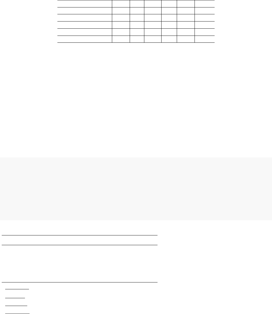
kableExtra also provides a few inline plotting tools. Right now, there are spec_hist, spec_boxplot, and

spec_plot. One key feature is that by default, the limits of every subplots are ﬁxed so you can compare

across rows.

mpg_list <- split(mtcars$mpg, mtcars$cyl)

disp_list <- split(mtcars$disp, mtcars$cyl)

inline_plot <- data.frame(cyl = c(4, 6, 8), mpg_box = "", mpg_hist = "",

mpg_line1 = "", mpg_line2 = "",

mpg_points1 = "", mpg_points2 = "", mpg_poly = "")

inline_plot %>%

kbl(booktabs = TRUE) %>%

kable_paper(full_width = FALSE) %>%

column_spec(2, image = spec_boxplot(mpg_list)) %>%

column_spec(3, image = spec_hist(mpg_list)) %>%

column_spec(4, image = spec_plot(mpg_list, same_lim = TRUE)) %>%

column_spec(5, image = spec_plot(mpg_list, same_lim = FALSE)) %>%

column_spec(6, image = spec_plot(mpg_list, type = "p")) %>%

cyl mpg_box mpg_hist mpg_line1 mpg_line2 mpg_points1 mpg_points2 mpg_poly

Variable Visualization

var 1

var 2

var 3

column_spec(7, image = spec_plot(mpg_list, disp_list, type = "p")) %>%

column_spec(8, image = spec_plot(mpg_list, polymin = 5))

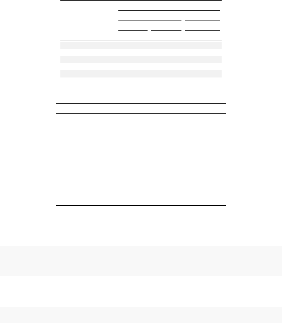
There is also a spec_pointrange function speciﬁcally designed for forest plots in regression tables. Of

course, feel free to use it for other purposes.

coef_table <- data.frame(

Variables = c("var 1", "var 2", "var 3"),

Coefficients = c(1.6, 0.2, -2.0),

Conf.Lower = c(1.3, -0.4, -2.5),

Conf.Higher = c(1.9, 0.6, -1.4)

)

data.frame(

Variable = coef_table$Variables,

Visualization = ""

) %>%

kbl(booktabs = T) %>%

kable_classic(full_width = FALSE) %>%

column_spec(2, image = spec_pointrange(

x = coef_table$Coefficients,

xmin = coef_table$Conf.Lower,

xmax = coef_table$Conf.Higher,

vline = 0)

)

Row spec

Similar with column_spec, you can deﬁne speciﬁcations for rows. Currently, you can either bold or italicize

an entire row. Note that, similar to other row-related functions in kableExtra, for the position of the target

row, you don’t need to count in header rows or the group labeling rows.

kbl(dt, booktabs = T) %>%

kable_styling("striped", full_width = F) %>%

column_spec(7, border_left = T, bold = T) %>%

row_spec(1, strikeout = T) %>%

row_spec(3:5, bold = T, color = "white", background = "black")

mpg cyl disp hp drat wt

Mazda RX4 21.0 6 160 110 3.90 2.620

Mazda RX4 Wag 21.0 6 160 110 3.90 2.875

Datsun 710 22.8 4 108 93 3.85 2.320

Hornet 4 Drive 21.4 6 258 110 3.08 3.215

Hornet Sportabout 18.7 8 360 175 3.15 3.440

mpg

cyl

disp

drat

Mazda RX4 21.0 6 160 110 3.90 2.620

Mazda RX4 Wag 21.0 6 160 110 3.90 2.875

Datsun 710 22.8 4 108 93 3.85 2.320

Hornet 4 Drive 21.4 6 258 110 3.08 3.215

Hornet Sportabout 18.7 8 360 175 3.15 3.440

Header Rows

One special case of row_spec is that you can specify the format of the header row via row_spec(row = 0,

...).

kbl(dt, booktabs = T, align = "c") %>%

kable_styling(latex_options = "striped", full_width = F) %>%

row_spec(0, angle = 45)

Cell/Text Speciﬁcation

Key Update: As said before, if you are using kableExtra 1.2+, you are now recom-

mended to used column_spec to do conditional formatting.

Function cell_spec is introduced in version 0.6.0 of kableExtra. Unlike column_spec and row_spec, this

function is designed to be used before the data.frame gets into the kable function. Comparing

with ﬁguring out a list of 2 dimensional indexes for targeted cells, this design is way easier to learn and use,

and it ﬁts perfectly well with dplyr’s mutate and summarize functions. With this design, there are two things

to be noted: * Since cell_spec generates raw HTML or LaTeX code, make sure you remember to put escape

= FALSE in kable. At the same time, you have to escape special symbols including % manually by yourself *

cell_spec needs a way to know whether you want html or latex. You can specify it locally in function or

globally via the options(knitr.table.format = "latex") method as suggested at the beginning. If you

don’t provide anything, this function will output as HTML by default.

Currently, cell_spec supports features including bold, italic, monospace, text color, background color, align,

font size & rotation angle. More features may be added in the future. Please see function documentations

as reference.

Conditional logic

It is very easy to use cell_spec with conditional logic. Here is an example.

car mpg cyl

Mazda RX4 21

Mazda RX4 Wag 21

Datsun 710 22.8

Hornet 4 Drive 21.4

Hornet Sportabout 18.7

Valiant 18.1

Duster 360 14.3

Merc 240D 24.4

Merc 230 22.8

Merc 280 19.2

cs_dt <- mtcars[1:10, 1:2]

cs_dt$car = row.names(cs_dt)

row.names(cs_dt) <- NULL

cs_dt$mpg = cell_spec(cs_dt$mpg, color = ifelse(cs_dt$mpg > 20, "red", "blue"))

cs_dt$cyl = cell_spec(

cs_dt$cyl, color = "white", align = "c", angle = 45,

background = factor(cs_dt$cyl, c(4, 6, 8), c("#666666", "#999999", "#BBBBBB")))

cs_dt <- cs_dt[c("car", "mpg", "cyl")]

kbl(cs_dt, booktabs = T, escape = F) %>%

kable_paper("striped", full_width = F)

# You can also do this with dplyr and use one pipe from top to bottom

# mtcars[1:10, 1:2] %>%

# mutate(

# car = row.names(.),

# mpg = cell_spec(mpg, "html", color = ifelse(mpg > 20, "red", "blue")),

# cyl = cell_spec(cyl, "html", color = "white", align = "c", angle = 45,

# background = factor(cyl, c(4, 6, 8),

# c("#666666", "#999999", "#BBBBBB")))

# ) %>%

# select(car, mpg, cyl) %>%

# kbl(format = "html", escape = F) %>%

# kable_styling("striped", full_width = F)

Visualize data with Viridis Color

This package also comes with a few helper functions, including spec_color, spec_font_size & spec_angle.

These functions can rescale continuous variables to certain scales. For example, function spec_color would

map a continuous variable to any viridis color palettes. It oﬀers a very visually impactful representation in

a tabular format.

vs_dt <- iris[1:10, ]

vs_dt[1:4] <- lapply(vs_dt[1:4], function(x) {

cell_spec(x, bold = T,

color = spec_color(x, end = 0.9),

font_size = spec_font_size(x))

Sepal.Length Sepal.Width Petal.Length Petal.Width Species

5.1 3.5 1.4 0.2 setosa

4.9 3 1.4 0.2 setosa

4.7 3.2 1.3 0.2 setosa

4.6 3.1 1.5 0.2 setosa

5 3.6 1.4 0.2 setosa

5.4 3.9 1.7 0.4 setosa

4.6 3.4 1.4 0.3 setosa

5 3.4 1.5 0.2 setosa

4.4 2.9 1.4 0.2 setosa

4.9 3.1 1.5 0.1 setosa

})

vs_dt[5] <- cell_spec(vs_dt[[5]], color = "white", bold = T,

background = spec_color(1:10, end = 0.9, option = "A", direction = -1))

kbl(vs_dt, booktabs = T, escape = F, align = "c") %>%

kable_classic("striped", full_width = F)

# Or dplyr ver

# iris[1:10, ] %>%

# mutate_if(is.numeric, function(x) {

# cell_spec(x, bold = T,

# color = spec_color(x, end = 0.9),

# font_size = spec_font_size(x))

# }) %>%

# mutate(Species = cell_spec(

# Species, color = "white", bold = T,

# background = spec_color(1:10, end = 0.9, option = "A", direction = -1)

# )) %>%

# kable(escape = F, align = "c") %>%

# kable_styling(c("striped", "condensed"), full_width = F)

Text Speciﬁcation

If you check the results of cell_spec, you will ﬁnd that this function does nothing more than wrapping

the text with appropriate HTML/LaTeX formatting syntax. The result of this function is just a vector of

character strings. As a result, when you are writing a rmarkdown document or write some text in shiny apps,

if you need extra markups other than bold or italic, you may use this function to color, change font

size or

rotate

your text.

An aliased function text_spec is also provided for a more literal writing experience. The only diﬀerence

is that in LaTeX, unless you specify latex_background_in_cell = FALSE (default is TRUE) in cell_spec,

it will deﬁne cell background color as \cellcolor{}, which doesn’t work outside of a table, while for

text_spec, the default value for latex_background_in_cell is FALSE.

sometext <- strsplit(paste0(

"You can even try to make some crazy things like this paragraph. ",

"It may seem like a useless feature right now but it's so cool ",

"and nobody can resist. ;)"

Group 1 Group 2 Group 3

mpg cyl disp hp drat wt

Mazda RX4 21.0 6 160 110 3.90 2.620

Mazda RX4 Wag 21.0 6 160 110 3.90 2.875

Datsun 710 22.8 4 108 93 3.85 2.320

Hornet 4 Drive 21.4 6 258 110 3.08 3.215

Hornet Sportabout 18.7 8 360 175 3.15 3.440

), " ")[[1]]

text_formatted <- paste(

text_spec(sometext, color = spec_color(1:length(sometext), end = 0.9),

font_size = spec_font_size(1:length(sometext), begin = 5, end = 20)),

collapse = " ")

# To display the text, type `r text_formatted` outside of the chunk

You can even try to make some crazy things like this paragraph. It may seem like a useless feature right

now but it’s so cool and nobody can resist. ;)

Grouped Columns / Rows

Add header rows to group columns

Tables with multi-row headers can be very useful to demonstrate grouped data. To do that, you can pipe

your kable object into add_header_above(). The header variable is supposed to be a named character with

the names as new column names and values as column span. For your convenience, if column span equals

to 1, you can ignore the =1 part so the function below can be written as ‘add_header_above(c(” “,”Group

1” = 2, “Group 2” = 2, “Group 3” = 2)).

kbl(dt, booktabs = T) %>%

kable_styling() %>%

add_header_above(c(" " = 1, "Group 1" = 2, "Group 2" = 2, "Group 3" = 2))

In fact, if you want to add another row of header on top, please feel free to do so. Also, since kableExtra

0.3.0, you can specify bold & italic as you do in row_spec().

kbl(dt, booktabs = T) %>%

kable_styling(latex_options = "striped") %>%

add_header_above(c(" ", "Group 1" = 2, "Group 2" = 2, "Group 3" = 2)) %>%

add_header_above(c(" ", "Group 4" = 4, "Group 5" = 2)) %>%

add_header_above(c(" ", "Group 6" = 6), bold = T, italic = T)

Group rows via labeling

Sometimes we want a few rows of the table being grouped together. They might be items under the same

topic (e.g., animals in one species) or just diﬀerent data groups for a categorical variable (e.g., age < 40, age

> 40). With the function pack_rows/group_rows() in kableExtra, this kind of task can be completed in

Group 6

Group 4 Group 5

Group 1 Group 2 Group 3

mpg cyl disp hp drat wt

Mazda RX4 21.0 6 160 110 3.90 2.620

Mazda RX4 Wag 21.0 6 160 110 3.90 2.875

Datsun 710 22.8 4 108 93 3.85 2.320

Hornet 4 Drive 21.4 6 258 110 3.08 3.215

Hornet Sportabout 18.7 8 360 175 3.15 3.440

Table 3: Group Rows

mpg cyl disp hp drat wt

Mazda RX4 21.0 6 160.0 110 3.90 2.620

Mazda RX4 Wag 21.0 6 160.0 110 3.90 2.875

Datsun 710 22.8 4 108.0 93 3.85 2.320

Group 1

Hornet 4 Drive 21.4 6 258.0 110 3.08 3.215

Hornet Sportabout 18.7 8 360.0 175 3.15 3.440

Valiant 18.1 6 225.0 105 2.76 3.460

Duster 360 14.3 8 360.0 245 3.21 3.570

Group 2

Merc 240D 24.4 4 146.7 62 3.69 3.190

Merc 230 22.8 4 140.8 95 3.92 3.150

Merc 280 19.2 6 167.6 123 3.92 3.440

one line. Please see the example below. Note that when you count for the start/end rows of the group, you

don’t need to count for the header rows nor other group label rows. You only need to think about the row

numbers in the “original R dataframe”.

kbl(mtcars[1:10, 1:6], caption = "Group Rows", booktabs = T) %>%

kable_styling() %>%

pack_rows("Group 1", 4, 7) %>%

pack_rows("Group 2", 8, 10)

In case some users need it, you can deﬁne your own gapping spaces between the group labeling row and

previous rows. The default value is 0.5em.

kbl(dt, booktabs = T) %>%

pack_rows("Group 1", 4, 5, latex_gap_space = "2em")

mpg cyl disp hp drat wt

Mazda RX4 21.0 6 160 110 3.90 2.620

Mazda RX4 Wag 21.0 6 160 110 3.90 2.875

Datsun 710 22.8 4 108 93 3.85 2.320

Group 1

Hornet 4 Drive 21.4 6 258 110 3.08 3.215

Hornet Sportabout 18.7 8 360 175 3.15 3.440

If you prefer to build multiple groups in one step, you can use the short-hand index option. Basically, you

can use it in the same way as you use add_header_above. However, since group_row only support one layer

of grouping, you can’t add multiple layers of grouping header as you can do in add_header_above.

kbl(mtcars[1:10, 1:6], caption = "Group Rows", booktabs = T) %>%

kable_styling() %>%

pack_rows(index=c(" " = 3, "Group 1" = 4, "Group 2" = 3))

# Not evaluated. The code above should have the same result as the first example in this section.

Note that kable has a relatively special feature to handle align and it may bring troubles to you if you are

not using it correctly. In the documentation of the align argument of kable, it says:

If length(align) == 1L, the string will be expanded to a vector of individual letters, e.g. 'clc'

becomes c('c', 'l', 'c'), unless the output format is LaTeX.

For example,

kbl(mtcars[1:2, 1:2], align = c("cl"))

# \begin{tabular}{l|cl|cl} # Note the column alignment here

# \hline

# & mpg & cyl\\

# ...

LaTeX, somehow shows surprisingly high tolerance on that, which is quite unusual. As a result, it won’t

throw an error if you are just using kable to make some simple tables. However, when you use kableExtra

to make some advanced modiﬁcation, it will start to throw some bugs. As a result, please try to form a habit

of using a vector in the align argument for kable (tip: you can use rep function to replicate elements. For

example, c("c", rep("l", 10))).

Row indentation

Unlike pack_rows(), which will insert a labeling row, sometimes we want to list a few sub groups under a

total one. In that case, add_indent() is probably more appropriate.

kbl(dt, booktabs = T) %>%

add_indent(c(1, 3, 5))

mpg cyl disp hp drat wt

Mazda RX4 21.0 6 160 110 3.90 2.620

Mazda RX4 Wag 21.0 6 160 110 3.90 2.875

Datsun 710 22.8 4 108 93 3.85 2.320

Hornet 4 Drive 21.4 6 258 110 3.08 3.215

Hornet Sportabout 18.7 8 360 175 3.15 3.440

You can also specify the width of the indentation by the level_of_indent option. At the same time, if you

want to indent every column, you can choose to turn on all_cols. Note that if a column is right aligned,

you probably won’t be able to see the eﬀect.

kbl(dt, booktabs = T, align = "l") %>%

add_indent(c(1, 3, 5), level_of_indent = 2, all_cols = T)

mpg cyl disp hp drat wt

Mazda RX4 21.0 6 160 110 3.90 2.620

Mazda RX4 Wag 21.0 6 160 110 3.90 2.875

Datsun 710 22.8 4 108 93 3.85 2.320

Hornet 4 Drive 21.4 6 258 110 3.08 3.215

Hornet Sportabout 18.7 8 360 175 3.15 3.440

Group rows via multi-row cell

Function pack_rows is great for showing simple structural information on rows but sometimes people

may need to show structural information with multiple layers. When it happens, you may consider us-

ing collapse_rows instead, which will put repeating cells in columns into multi-row cells.

In LaTeX, collapse_rows adds some extra hlines to help diﬀerentiate groups. You can customize this

behavior using the latex_hline argument. You can choose from full (default), major and none.

Vertical alignment of cells (with the default row_group_label_position = "identity")) is controlled by

the valign option. You can choose from “top”, “middle” (default) and “bottom”. Be cautious that the

vertical alignment option was only introduced in multirow in 2016. If you are using a legacy LaTeX dis-

tribution, you will run into trouble if you set valign to be either “top” or “bottom”. Alternatively, use

row_group_label_position = "first", which will put the row group labels into the ﬁrst row without

using the \multirow LaTeX command at all.

collapse_rows_dt <- data.frame(C1 = c(rep("a", 10), rep("b", 5)),

C2 = c(rep("c", 7), rep("d", 3), rep("c", 2), rep("d", 3)),

C3 = 1:15,

C4 = sample(c(0,1), 15, replace = TRUE))

kbl(collapse_rows_dt, booktabs = T, align = "c") %>%

column_spec(1, bold=T) %>%

collapse_rows(columns = 1:2, latex_hline = "major", row_group_label_position = "first")

C1 C2 C3 C4

a c 1 1

2 0

3 0

4 1

5 1

6 1

7 0

d 8 0

9 1

10 1

b c 11 0

12 1

d 13 1

14 0

15 1

Right now, you can’t automatically make striped rows based on collapsed rows but you can do it manually

via the extra_latex_after option in row_spec. This feature is not oﬃcially supported. I’m only document

it here if you want to give it a try.

kbl(collapse_rows_dt[-1], align = "c", booktabs = T) %>%

column_spec(1, bold = T, width = "5em") %>%

row_spec(c(1:7, 11:12) - 1, extra_latex_after = "\\rowcolor{gray!6}") %>%

collapse_rows(1, latex_hline = "none")

C2 C3 C4

1 1

2 0

3 0

4 1

5 1

6 1

7 0

8 0

9 1d

10 1

11 0

12 1

13 1

14 0d

15 1

When there are too many layers, sometimes the table can become too wide. You can choose to stack the

ﬁrst few layers by setting row_group_label_position to stack.

collapse_rows_dt <- expand.grid(

District = sprintf('District %s', c('1', '2')),

City = sprintf('City %s', c('1', '2')),

State = sprintf('State %s', c('a', 'b')),

Country = sprintf('Country with a long name %s', c('A', 'B'))

)

collapse_rows_dt <- collapse_rows_dt[c("Country", "State", "City", "District")]

collapse_rows_dt$C1 = rnorm(nrow(collapse_rows_dt))

collapse_rows_dt$C2 = rnorm(nrow(collapse_rows_dt))

kbl(collapse_rows_dt,

booktabs = T, align = "c", linesep = '') %>%

collapse_rows(1:3, row_group_label_position = 'stack')

City District C1 C2

Country with a long name A

State a

City 1 District 1 0.8497568 -0.5419112

District 2 0.2831570 -1.5060217

City 2 District 1 -1.7532639 0.5432794

District 2 -0.2305938 -1.3727976

State b

City 1 District 1 -0.3414902 -0.4459881

District 2 -0.5041269 0.7015499

City 2 District 1 1.0522049 1.0731569

District 2 -0.9046838 0.2800722

Country with a long name B

State a

City 1 District 1 -0.6697488 -0.9879278

District 2 -1.5457403 -0.1835274

City 2 District 1 0.4152464 0.3018637

District 2 -0.1996067 -0.3375753

State b

City 1 District 1 2.4521916 1.3455051

District 2 0.2088972 -0.9741941

City 2 District 1 -1.0817609 1.7361157

District 2 0.1868137 -1.8330631

To better distinguish diﬀerent layers, you can format the each layer using row_group_label_fonts. You

can also customize the hlines to better diﬀerentiate groups.

row_group_label_fonts <- list(

list(bold = T, italic = T),

list(bold = F, italic = F)

)

kbl(collapse_rows_dt,

booktabs = T, align = "c", linesep = '') %>%

column_spec(1, bold=T) %>%

collapse_rows(1:3, latex_hline = 'custom', custom_latex_hline = 1:3,

row_group_label_position = 'stack',

row_group_label_fonts = row_group_label_fonts)

City District C1 C2

Country with a long name A

State a

City 1 District 1 0.8497568 -0.5419112

District 2 0.2831570 -1.5060217

City 2 District 1 -1.7532639 0.5432794

District 2 -0.2305938 -1.3727976

State b

City 1 District 1 -0.3414902 -0.4459881

District 2 -0.5041269 0.7015499

City 2 District 1 1.0522049 1.0731569

District 2 -0.9046838 0.2800722

Country with a long name B

State a

City 1 District 1 -0.6697488 -0.9879278

District 2 -1.5457403 -0.1835274

City 2 District 1 0.4152464 0.3018637

District 2 -0.1996067 -0.3375753

State b

City 1 District 1 2.4521916 1.3455051

District 2 0.2088972 -0.9741941

City 2 District 1 -1.0817609 1.7361157

District 2 0.1868137 -1.8330631

Table Footnote

Now it’s recommended to use the new footnote function instead of add_footnote to make table

footnotes.

Documentations for add_footnote can be found here.

There are four notation systems in footnote, namely general, number, alphabet and symbol. The last

three types of footnotes will be labeled with corresponding marks while general won’t be labeled. You can

pick any one of these systems or choose to display them all for fulﬁlling the APA table footnotes requirements.

kbl(dt, align = "c") %>%

kable_styling(full_width = F) %>%

footnote(general = "Here is a general comments of the table. ",

number = c("Footnote 1; ", "Footnote 2; "),

alphabet = c("Footnote A; ", "Footnote B; "),

symbol = c("Footnote Symbol 1; ", "Footnote Symbol 2")

)

mpg cyl disp hp drat wt

Mazda RX4 21.0 6 160 110 3.90 2.620

Mazda RX4 Wag 21.0 6 160 110 3.90 2.875

Datsun 710 22.8 4 108 93 3.85 2.320

Hornet 4 Drive 21.4 6 258 110 3.08 3.215

Hornet Sportabout 18.7 8 360 175 3.15 3.440

Note:

Here is a general comments of the table.

Footnote 1;

Footnote 2;

Footnote A;

Footnote B;

Footnote Symbol 1;

†

Footnote Symbol 2

You can also specify title for each category by using the ***_title arguments. Default value for

general_title is “Note:” and “ ” for the rest three. You can also change the order using footnote_order.

You can even display footnote as chunk texts (default is as a list) using footnote_as_chunk. The font

format of the titles are controlled by title_format with options including “italic” (default), “bold” and

“underline”.

kbl(dt, align = "c", booktabs = T) %>%

footnote(general = "Here is a general comments of the table. ",

number = c("Footnote 1; ", "Footnote 2; "),

alphabet = c("Footnote A; ", "Footnote B; "),

symbol = c("Footnote Symbol 1; ", "Footnote Symbol 2"),

general_title = "General: ", number_title = "Type I: ",

alphabet_title = "Type II: ", symbol_title = "Type III: ",

footnote_as_chunk = T, title_format = c("italic", "underline")

)

mpg cyl disp hp drat wt

Mazda RX4 21.0 6 160 110 3.90 2.620

Mazda RX4 Wag 21.0 6 160 110 3.90 2.875

Datsun 710 22.8 4 108 93 3.85 2.320

Hornet 4 Drive 21.4 6 258 110 3.08 3.215

Hornet Sportabout 18.7 8 360 175 3.15 3.440

General: Here is a general comments of the table.

Type I:

Footnote 1;

Footnote 2;

Type II:

Footnote A;

Footnote B;

Type III:

Footnote Symbol 1;

†

Footnote Symbol 2

If you need to add footnote marks in a table, you need to do it manually (no fancy) using

footnote_marker_***(). Remember that similar with cell_spec, you need to tell this function whether

you want it to do it in HTML (default) or LaTeX. You can set it for all using the knitr.table.format global

option. Also, if you have ever used footnote_marker_***(), you need to put escape = F in your kable

function to avoid escaping of special characters. Note that if you want to use these footnote_marker

functions in kableExtra functions like pack_rows (for the row label) or add_header_above, you need to

set double_escape = T and escape = F in those functions. I’m trying to ﬁnd other ways around. Please

let me know if you have a good idea and are willing to contribute.

Table 4: s

mpg cyl disp hp drat wt

Mazda RX4 21.0 6 160 110 3.90 2.620

Mazda RX4 Wag 21.0 6 160 110 3.90 2.875

Datsun 710 22.8 4 108 93 3.85 2.320

Hornet 4 Drive 21.4 6 258 110 3.08 3.215

Hornet Sportabout 18.7 8 360 175 3.15 3.440

Note:

Here is a very very very very very very very very very very

very very very very very very very very very very long foot-

note

dt_footnote <- dt

names(dt_footnote)[2] <- paste0(names(dt_footnote)[2],

# That "latex" can be eliminated if defined in global

footnote_marker_symbol(1, "latex"))

row.names(dt_footnote)[4] <- paste0(row.names(dt_footnote)[4],

footnote_marker_alphabet(1))

kbl(dt_footnote, align = "c", booktabs = T,

# Remember this escape = F

escape = F) %>%

footnote(alphabet = "Footnote A; ",

symbol = "Footnote Symbol 1; ",

alphabet_title = "Type II: ", symbol_title = "Type III: ",

footnote_as_chunk = T)

mpg cyl

disp hp drat wt

Mazda RX4 21.0 6 160 110 3.90 2.620

Mazda RX4 Wag 21.0 6 160 110 3.90 2.875

Datsun 710 22.8 4 108 93 3.85 2.320

Hornet 4 Drive

21.4 6 258 110 3.08 3.215

Hornet Sportabout 18.7 8 360 175 3.15 3.440

Type II:

Footnote A;

Type III:

Footnote Symbol 1;

If your table footnote is very long, please consider to put your table in a ThreePartTable frame. Note that,

in kableExtra version <= 0.7.0, we were using threeparttable but since kableExtra 0.8.0, we start to use

ThreePartTable from threeparttablex instead. ThreePartTable supports both the longtable and tabu

environments.

kbl(dt, align = "c", booktabs = T, caption = "s") %>%

footnote(general = "Here is a very very very very very very very very very very very very very very very very very very very very long footnote",

threeparttable = T)

LaTeX Only Features

Linebreak processor

Unlike in HTML, where you can use <br> at any time, in LaTeX, it’s actually quite diﬃcult to make a

linebreak in a table. Therefore I created the linebreak function to facilitate this process. Please see the

Best Practice for Newline in LaTeX Table for details.

dt_lb <- data.frame(

Item = c("Hello\nWorld", "This\nis a cat"),

Value = c(10, 100)

)

dt_lb$Item = linebreak(dt_lb$Item)

# Or you can use

# dt_lb <- dt_lb %>%

# mutate_all(linebreak)

dt_lb %>%

kbl(booktabs = T, escape = F,

col.names = linebreak(c("Item\n(Name)", "Value\n(Number)"), align = "c"))

Item

(Name)

Value

(Number)

Hello

World

This

is a cat

100

At the same time, since kableExtra 0.8.0, all kableExtra functions that have some contents input (such

as footnote or pack_rows) will automatically convert \n to linebreaks for you in both LaTeX and HTML.

Table on a Landscape Page

Sometimes when we have a wide table, we want it to sit on a designated landscape page. The new function

landscape() can help you on that. Unlike other functions, this little function only serves LaTeX and doesn’t

have a HTML side.

kbl(dt, caption = "Demo Table (Landscape)[note]", booktabs = T) %>%

kable_styling(latex_options = c("hold_position")) %>%

add_header_above(c(" ", "Group 1[note]" = 3, "Group 2[note]" = 3)) %>%

add_footnote(c("This table is from mtcars",

"Group 1 contains mpg, cyl and disp",

"Group 2 contains hp, drat and wt"),

notation = "symbol") %>%

pack_rows("Group 1", 4, 5) %>%

landscape()

Table 5: Demo Table (Landscape)

Group 1

†

Group 2

‡

mpg cyl disp hp drat wt

Mazda RX4 21.0 6 160 110 3.90 2.620

Mazda RX4 Wag 21.0 6 160 110 3.90 2.875

Datsun 710 22.8 4 108 93 3.85 2.320

Group 1

Hornet 4 Drive 21.4 6 258 110 3.08 3.215

Hornet Sportabout 18.7 8 360 175 3.15 3.440

This table is from mtcars

†

Group 1 contains mpg, cyl and disp

‡

Group 2 contains hp, drat and wt

Decimal Alignment

Decimal alignment has been a requested feature by many LaTeX users. However, since the syntax for either

siunitx or dcolumn are a little diﬀerent, it is sort of diﬃcult to integrate them into the pipeline of this

package without breaking other features. If you need this feature, Brandon Bertelsen (@1beb) provided

a very nice solution on Github (https://github.com/haozhu233/kableExtra/issues/174, thanks). Here is a

working example.

In the header-includes section of the YAML header, include the following settings. If you need diﬀerent

rounding options, you can make changes here.

\usepackage{siunitx}

\newcolumntype{d}{S[table-format=3.2]}

For your table, you need to modify the column names and use d to as the align options.

# not evaluated

k <- mtcars[1:10,1:5]

names(k) <- paste("{", names(k), "}")

kableExtra::kable(

k, "latex", booktabs = TRUE, longtable = TRUE,

align = c("l", rep("d", 4)), linesep = "", escape = FALSE) %>%

kable_styling(full_width=FALSE)

Use LaTeX table in HTML or Word

If you want to save a LaTeX table to a image, you may consider using save_kable(). We also provide an

as_image() function as a convenience wrapper for save_kable(). It will save the image to a temp location.

Note that this feature requires you to have magick installed (install.packages("magick")). Also, if you

are planning to use it on Windows, you need to install Ghostscript. This feature may not work if you are

using tinytex. If you are using tinytex, please consider using other alternatives to this function.

# Not evaluated.

# The code below will automatically include the image in the R Markdown document

kbl(dt, booktabs = T) %>%

column_spec(1, bold = T) %>%

as_image()

# If you want to save the image locally, just provide a name

kbl(dt, booktabs = T) %>%

column_spec(1, bold = T) %>%

save_kable("my_latex_table.png")

From other packages

Since the structure of kable is relatively simple, it shouldn’t be too diﬃcult to convert HTML or LaTeX

tables generated by other packages to a kable object and then use kableExtra to modify the outputs. If

you are a package author, feel free to reach out to me and we can collaborate.

tables

The latest version of tables comes with a toKable() function, which is compatible with functions in

kableExtra (>=0.9.0).

xtable

For xtable users, if you want to use kableExtra functions on that, check out this xtable2kable() function

shipped with kableExtra 1.0. I personally have been using this function to place table caption below tables

and solve some tricky case when I use tufte_handout.

# Not evaluating

xtable::xtable(mtcars[1:4, 1:4], caption = "Hello xtable") %>%

xtable2kable() %>%

column_spec(1, color = "red")