Stock Returns and Inflation Redux: An Explanation from Monetary Policy in Advanced and Emerging Markets, WP/21/219, August 2021

WP/21/219

Stock Returns and Inflation Redux: An Explanation from

Monetary Policy in Advanced and Emerging Markets

by Zhongxia Zhang

IMF Working Papers describe research in progress by the author(s) and are published to

elicit comments and to encourage debate. The views expressed in IMF Working Papers are

those of the author(s) and do not necessarily represent the views of the IMF, its Executive

Board, or IMF management.

IMF Working Paper

European Department

Stock Returns and Inflation Redux: An Explanation from Monetary Policy in

Advanced and Emerging Markets

Prepared by Zhongxia Zhang

Authorized for distribution by Rachel van Elkan

August 2021

Abstract

Classical theories of monetary economics predict that real stock returns are negatively

correlated with inflation when monetary policy is countercyclical. Previous empirical

studies mostly focus on a small group of developed countries or a few countries with

hyperinflation. In this paper, I examine the stock return-inflation relation under different

monetary policy regimes and conditions using an expanded dataset of 71 economies.

Empirical evidence suggests that the stock return-inflation relation is partially driven by

monetary policy. If a country’s monetary authority conducts a more countercyclical

monetary policy, the stock return-inflation relation becomes more negative. In addition,

the results differ by monetary policy framework. In exchange rate anchor countries, stock

markets do not respond to monetary policy cyclicality. In inflation targeting countries,

stock markets react more strongly to inflation. A key contribution of this paper is to

classify inflation targeters by their behaviors, and illustrate that behavior matters in

shaping market perceptions: markets react to inflation and monetary policy cyclicality

when central banks are able to control inflation within their target bands. In this case

markets are sensitive to inflation dynamics when inflation is above the announced target

bands. Finally, when monetary policy is constrained by the Zero Lower Bound (ZLB), a

structural break is introduced and real stock returns no longer respond to inflation and

monetary policy cyclicality.

JEL Classification Numbers: G12, E31, E52.

Keywords: Stock Return, Inflation, Monetary Policy.

Author’s E-Mail Address: zzhang2@imf.org

IMF Working Papers describe research in progress by the author(s) and are published to

elicit comments and to encourage debate. The views expressed in IMF Working Papers are

those of the author(s) and do not necessarily represent the views of the IMF, its Executive

Board, or IMF management.

Stock Returns and Inﬂation Redux: An

Explanation from Monetary Policy in Advanced

and Emerging Markets

∗

Zhongxia Zhang

International Monetary Fund

August 4, 2021

Abstract

Classical theories of monetary economics predict that real stock returns are neg-

atively correlated with inﬂation when monetary policy is countercyclical. Previous

empirical studies mostly focus on a small group of developed countries or a few coun-

tries with hyperinﬂation. In this paper, I examine the stock return-inﬂation relation

under diﬀerent monetary policy regimes and conditions using an expanded dataset

of 71 economies. Empirical evidence suggests that the stock return-inﬂation relation

is partially driven by monetary policy. If a country’s monetary authority conducts

a more countercyclical monetary policy, the stock return-inﬂation relation becomes

more negative. In addition, the results diﬀer by monetary policy framework. In

exchange rate anchor countries, stock markets do not respond to monetary policy

∗

Zhang: European Department, International Monetary Fund, 700 19th Street, N.W., Washing-

ton, D.C. 20431 (email: [email protected]). I am grateful to Jay Shambaugh, Graciela Kaminsky,

Tara Sinclair, Chao Wei, Michael Bradley, Pamela Labadie, Frederick Joutz, Robert Phillips, Va-

lerie Ramey, Carl Walsh, Aart Kraay, Tamim Bayoumi, Rachel van Elkan, Xingwei Hu, Evridiki

Tsounta, Dong Wu, Xin Xu, Peichu Xie, Dun Jia, and participants at the 2018 Asian Meeting of

the Econometric Society, IMF EUR seminar, GWU Macro-International seminar, 3rd international

Workshop on Financial Markets and Nonlinear Dynamics, 22nd EBES Conference, Workshop on Fi-

nancial Econometrics and Empirical Modeling of Financial Markets, 43rd EEA Annual Conference

for their valuable comments. The views expressed in this paper are those of the author. All errors

are my own.

cyclicality. In inﬂation targeting countries, stock markets react more strongly to in-

ﬂation. A key contribution of this paper is to classify inﬂation targeters by their

behaviors, and illustrate that behavior matters in shaping market perceptions: mar-

kets react to inﬂation and monetary policy cyclicality when central banks are able

to control inﬂation within their target bands. In this case, markets are sensitive to

inﬂation dynamics when inﬂation is above the announced target bands. Finally, when

monetary policy is constrained by the Zero Lower Bound (ZLB), a structural break is

introduced and real stock returns no longer respond to inﬂation and monetary policy

cyclicality.

JEL Classiﬁcation: G12, E31, E52.

Keywords: Stock Return, Inﬂation, Monetary Policy.

1 Introduction

The subject of stock returns and inﬂation enjoys a decades-long research history.

Academic interests in this topic have waxed and waned with the importance of in-

ﬂation on the macroeconomy. The high inﬂation episodes in the 1970s have imposed

heavy costs on living standards and economic stability. Stock returns were dismal

during this period, which in turn sparked extensive studies in stock returns and in-

ﬂation. The COVID-19 pandemic has triggered renewed interest in the relationship

between stock returns and inﬂation. To mitigate the impact of the pandemic, central

banks and ﬁnance ministries around the world have taken unprecedented policy ac-

tions. While such actions were pivotal in preventing a free fall of the world economy

and supporting a robust recovery, there could be side eﬀects such as asset bubbles

and widening inequality. As Consumer Price Indices rebound strongly in many parts

of the world, concerns arise on whether the pick-up in inﬂation is temporary or per-

manent and the associated implications for the ﬁnancial markets.

The topic of stock returns and inﬂation covers a joint research area of ﬁnance and

macroeconomics. For ﬁnancial economists, the relationship between stock returns and

inﬂation quantiﬁes the extent to which stocks can hedge against inﬂation risk. It is

important for trading and risk management purposes. Monetary economists are keen

to understand whether inﬂation and monetary policy have any eﬀect on stock returns.

The stock market is a primary source of direct ﬁnancing for ﬁrms, and stock price

ﬂuctuations aﬀect real economic activity and ﬁnancial stability, including corporate

borrowing and investment decisions (Baker et al., 2003; Pastor and Veronesi, 2003),

and household consumption and saving decisions induced by changes in net worth.

Therefore, central banks that aim at stabilizing prices have to take into account the

eﬀects of inﬂation on asset returns.

Historically, real stock prices decline when inﬂation rises in developed countries.

Equity shares, which are claims on future output of ﬁrms, do not prove to be a good

hedge against inﬂation risk as researchers ﬁnd a negative correlation between real

stock return and inﬂation in the short run in developed countries. This phenomenon

has intrigued the economics profession to investigate why inﬂation as a nominal vari-

able has an impact on real stock prices or the real value of claims on physical assets.

Among various theories to explain the negative stock return-inﬂation correlation,

existing hypotheses in monetary economics assert that the negative relationship is a

result of central bank’s countercyclical policy reaction: when inﬂation rises, a central

bank that aims to maintain price stability and conducts countercyclical monetary

policy will lift its policy rate. Therefore, changes in inﬂation aﬀect real interest rates.

As the stock price is equal to the current value of all future cash ﬂows, an increase in

interest rate (discount rate) lowers the net present value of stocks. In addition, higher

interest rates lead to larger borrowing costs for ﬁrms, increase the attractiveness of

competing assets such as bonds and deposits, dry up liquidity in the stock market,

and put downward pressures on stock returns.

Previous work on this issue mostly focuses on either one country (Fama, 1981), a

small group of industrialized countries, with just a few studies focusing on emerging

markets (Spyrou, 2004; Gultekin, 1983 and Erb et al., 1995 are exceptions), despite

the rising importance of emerging markets (Cubeddu et al., 2014). Gultekin (1983)

investigates stock returns and inﬂation in 26 countries for the postwar period, and

Erb et al. (1995) study stock returns and inﬂation in 41 developed and emerging eq-

uity markets over 22 years. These studies appear less representative given the rapidly

changing developments in the international monetary and ﬁnancial system, especially

the rise of emerging market economies, as well as inﬂation developments from previ-

ous hyperinﬂation concerns have been superseded by the subsequent deﬂation risk.

Indeed, in recent years, policymakers and investors are increasingly wary of stock

market spillover eﬀects from emerging markets to the rest of the world, while more

emerging markets’ central banks are moving towards inﬂation targeting regimes.

This paper aims to revisit the important policy question of how monetary policy

aﬀects the way stock returns react to inﬂation. In this paper, I expand the research

to a quarterly panel dataset of 71 advanced and emerging economies over a period of

35 years. This dataset contains not only rich information on stock returns and inﬂa-

tion, but also substantial variations of other macroeconomic variables and ﬁnancial

indicators. It makes comparisons among countries and across several monetary policy

dimensions possible. This paper dissects monetary policy into diﬀerent regimes and

conditions to understand its role on stock returns and inﬂation (Figure 1). It focuses

on three key elements of monetary policy: monetary policy cyclicality, monetary pol-

icy framework and monetary policy ﬂexibility. Doing so can show a comprehensive

picture of the eﬀectiveness of monetary policy in driving the stock return-inﬂation

Figure 1: Key Monetary Policy Elements that Aﬀect Stock Returns and Inﬂation

relations. To the best of my knowledge, this is the ﬁrst paper that studies stock re-

turns and inﬂation, tests hypotheses of monetary policy cyclicality in the literature,

and documents diﬀerences between the advanced and emerging markets from such a

broad set of countries. It examines the outcomes of monetary policy frameworks with

an emphasis on inﬂation targeters’ behaviors, as well as the Zero Lower Bound.

I ﬁrst examine the stock return-inﬂation relationship based on monetary policy

cyclicality. I augment the panel regressions by including monetary policy cyclicality

measures and a monetary aggregate factor. To address the econometric issues of serial

correlation, heteroskedasticity, and cross-sectional dependence, I apply the Driscoll-

Kraay standard error estimators. By testing an existing hypothesis in the literature,

results conﬁrm that monetary policy cyclicality can partly explain why stock markets

respond diﬀerently to inﬂation. Results indicate that real stock returns decline when

inﬂation increases, with larger reactions to inﬂation in advanced markets than emerg-

ing markets. The diﬀerences between advanced and emerging markets are interesting

but they have not been highlighted enough in the literature before. They imply that

practitioners and policymakers in emerging markets should use caution when borrow-

ing the experience from advanced markets. Moreover, if a country pursues a more

countercyclical monetary policy, stock markets will react more negatively to inﬂation.

I then study the stock return-inﬂation relationship across monetary policy frame-

works. Under an exchange rate anchor regime, real stock returns do not pay attention

to the monetary policy cyclicality. In contrast, under an inﬂation targeting regime,

real stock returns react extremely negatively to inﬂation, compared to the baseline

ﬁndings. When central banks have the capacity to control inﬂation within their an-

nounced target bands, markets are sensitive to inﬂation dynamics when inﬂation is

above the target band. I show that inﬂation targeting countries exhibit a large degree

of heterogeneity regarding the amount of time inﬂation stays within the central bank’s

target bands. And stock markets do diﬀerentiate behavior by reacting diﬀerently to

inﬂation and monetary policy cyclicality.

Finally, I analyze the role of monetary policy ﬂexibility on stock return and in-

ﬂation. When the policy rate is constrained by the Zero Lower Bound, a structural

break is revealed and markets disregard inﬂation and monetary policy cyclicality. The

results illustrate how limited monetary policy ﬂexibility alters the way stock returns

react to inﬂation.

The remainder of the paper is organized as follows: Section 2 provides a brief

and selective literature review on previous studies. Section 3 documents the under-

lying data and presents some key stylized facts. Section 4 describes the analytical

framework and displays the main results from panel regressions. It examines the

role of monetary policy by testing an existing hypothesis in the literature. It also

runs augmented regressions and shows how monetary policy cyclicality shapes the

stock return-inﬂation relation. Diﬀerent monetary policy frameworks and the out-

come of Zero Lower Bound are also studied. Section 5 performs several robustness

checks. Section 6 discusses policy implications, possible avenues for future research,

and concludes.

2 Literature Review

It is empirically well documented in the literature that nominal stock returns re-

act negatively to inﬂation in the United States and several industrialized countries

(Lintner, 1975; Fama and Schwert, 1977; Fama, 1981). This is a long-standing phe-

nomenon that has attracted economists’ attention, because people do not expect real

stock return is aﬀected by a nominal variable such as inﬂation. According to the clas-

sical view of Irving Fisher (1930), expected nominal return on an asset should equal

the expected real return plus expected inﬂation. Therefore, stocks, which represent

claims on real output of ﬁrms, should be a good hedge against both expected and

unexpected inﬂation. In the “best of all possible worlds”, one should observe that

the nominal interest rate co- move in a one-to-one relationship with inﬂation if the

real interest rate is constant in the short term.

Research on the stock return-inﬂation relation from an international perspective

produce similar ﬁndings. Gultekin (1983) investigates the relation between common

stock returns and inﬂation in 26 countries for the postwar period, and shows that

the results do not support the Fisher Hypothesis. Erb et al. (1995) study inﬂation

and stock returns in 41 developed and emerging equity markets over 22 years and

document a signiﬁcant negative relation for most countries.

The empirical anomaly has sparked a number of hypotheses attempting to explain

the phenomenon, most notably the inﬂation illusion hypothesis (Modigliani and Cohn,

1979; Campbell and Vuolteenaho, 2004), the proxy hypothesis (Fama, 1981), the tax

hypothesis (Feldstein, 1980), the time-varying risk aversion hypothesis (Brandt and

Wang, 2003), and the sticky discount rate hypothesis (Katz et al., 2017). The inﬂation

illusion hypothesis proposed by Modigliani and Cohn (1979) states that stock market

investors fail to understand the eﬀect of inﬂation on nominal dividend growth rates

and extrapolate historical growth rates even in periods of changing inﬂation. From

a rational investor’s perspective, this implies that stock prices are undervalued when

inﬂation is high and overvalued when inﬂation is low. Campbell and Vuolteenaho

(2004) ﬁnd that the regression coeﬃcient of the mispricing component on inﬂation

is positively and statistically signiﬁcant, and their results provide strong support to

the inﬂation illusion hypothesis. Fama (1981) considers the negative correlation be-

tween stock returns and inﬂation as the consequence of proxy eﬀects. He explains in

his proxy hypothesis that there is no causal relationship between the two variables.

Instead, both variables are driven by real economic activity. Stock returns are de-

termined by forecasts of relevant real variables, and negative stock return-inﬂation

relations are induced by negative relations between real activity and inﬂation. The

negative stock return-inﬂation relations are induced by negative relations between

inﬂation and real activity which in turn are explained by a combination of money

demand theory and the quantity theory of money.

Feldstein (1980) argues that an important adverse eﬀect of increased inﬂation on

share prices results from basic features of the current U.S. tax laws, particularly his-

toric cost depreciation and the taxation on nominal capital gains. When prices rise,

the historic cost method of depreciation causes the real value of depreciation to fall

and real taxable proﬁts to be increased. As a result, real proﬁts net of the corporate

income tax vary inversely with inﬂation. Inﬂation further reduces net earnings by

imposing an additional tax on nominal capital gains. Therefore, inﬂation raises the

eﬀective tax rate on corporate income and lowers the share price. In a recent attempt,

Brandt and Wang (2003) put forward a time-varying risk aversion hypothesis. They

formulate a consumption-based asset pricing model in which aggregate risk aversion

is time-varying in response to news about consumption growth and inﬂation. They

document a robust correlation between aggregate risk aversion and unexpected inﬂa-

tion. Katz et al. (2017) investigate why local stock markets adjust slowly to changes

in local inﬂation. They ﬁnd that when the local rate of inﬂation increases, local in-

vestors subsequently earn lower real returns on local stocks, suggesting that the local

stock market investors use sticky long-run nominal discount rates that are too low

when inﬂation increases because they are slow to update the inﬂation expectations in

discount rates. They show that small amounts of stickiness in inﬂation expectations

are suﬃcient to match the real stock return predictability induced by inﬂation in the

data.

There is another strand of the literature that emphasizes the role of monetary

policy in determining stock returns and inﬂation. The rationale is that central banks

that are targeting inﬂation will respond to inﬂation shocks. As a result, the changing

stance of monetary policy prompts stock market revaluations. Sellin (2001) gives a

comprehensive review of the literature on the interaction between stock returns, inﬂa-

tion, and money growth, with a special emphasis on the role of monetary policy. Kaul

(1987) hypothesizes that the relation between stock returns and inﬂation is caused

by equilibrium processes in the monetary sector. He shows that the negative stock

return-inﬂation relations are caused by money demand and countercyclical money

supply eﬀects. Geske and Roll (1983) argue that this puzzling empirical phenomenon

is due to the ﬁscal and monetary linkage. Exogenous shocks in real output, signaled

by the stock market, induce changes in tax revenue, then the Treasury borrows more

and the central bank monetizes the increased debt. Rational investors adjust prices

accordingly without a delay. Using Markov regime-switching models, Chen (2007)

points out that monetary policy has asymmetric eﬀects on stock returns.

In a thought-provoking paper, Bakshi and Chen (1996) show that there exists a

negative correlation between real equity return and inﬂation within a general equi-

librium, unless both money growth is procyclical and its covariance with output

growth dominates the variance of output growth. In a Cash-in-Advance model, Boyle

and Peterson (1995) show that equity returns are negatively correlated with inﬂation

when monetary policy is countercyclical or weakly procyclical. In another equilibrium

monetary asset pricing model, Marshall (1992) predicts that the inﬂation-asset return

correlation will be more strongly negative when inﬂation is generated by ﬂuctuations

in real economic activity than when it is generated by monetary ﬂuctuations. In an

inﬂuential paper, Christiano et al. (2010) show that historically, inﬂation is low dur-

ing stock market booms in the United States and Japan. The authors use the concept

of a news shock, i.e., a disturbance to information about next period’s innovation in

technology, to interpret the evidence. They argue that an interest rate rule that is too

narrowly focused on inﬂation destabilizes asset markets and the broader economy.

The paper revisits the existing monetary economics hypotheses in the stock return-

inﬂation literature and contribute to the literature by highlighting the role of mon-

etary policy. It intends to conﬁrm monetary policy as a determining factor in the

stock return-inﬂation relationship based on empirical ﬁndings under diﬀerent mon-

etary policy regimes and conditions. It empirically conﬁrms that central banks can

shape the way stock markets react to inﬂation from three diﬀerent angles: mone-

tary policy cyclicality, monetary policy framework, and whether monetary policy is

constrained by the Zero Lower Bound. In addition, this paper contributes to the in-

ﬂation targeting literature by revealing that inﬂation targeting countries are diﬀerent.

Based on a stark comparison of central banks’ track record of controlling inﬂation,

results show that inﬂation targeting countries are heterogeneous and stock markets

diﬀerentiate inﬂation targeting countries by their behaviors.

3 Data Description and Stylized Facts

I compile a quarterly dataset using readily available data from the ﬁrst quarter of

1980 to the second quarter of 2015. The sample includes 71 economies, including 33

advanced markets and 38 emerging markets. It integrates data from the International

Monetary Fund (IMF), Bloomberg, Haver Analytics, Thomson Reuters Datastream,

Consensus Forecasts, and other sources. The dataset is an unbalanced panel, that is,

countries do not have the same number of observations in the study. For example, the

stock market has a long history in advanced markets, while for emerging markets it

is a recent phenomenon. The issue of data availability is also true for other variables.

The variable construction and data source of key variables are as follows (see

details in appendix). Equity index data is from Bloomberg, and nominal stock return

is the change in equity index logarithm from one year ago. Consumer price index

data is from the IMF’s INS database, and inﬂation is deﬁned as the change in the

Consumer Price Index (CPI) logarithm from one year ago. Real equity index is

derived by deﬂating nominal equity index by consumer price index accordingly, and

real stock return is the change in real equity price logarithm from one year ago.

Inﬂation forecasts are current-year and next-year market forecasts from Consensus

Forecasts. Industrial production data is obtained from combining Thomson Reuters

Datastream and the IMF’s data. M2, a measure of aggregate money supply, comes

from Haver Analytics and the IMF. Financial sector risk ratings are provided by the

International Country Risk Guide (ICRG). The United States three-month Treasury

bill yield rate in secondary markets is downloaded from the Board of Governors of

the Federal Reserve System. Finally, the VIX index is retrieved from Bloomberg.

Table 1 summarizes the basic statistics for key indicators used in this paper.

Nominal stock returns on average are 0.11, and the standard deviation is 0.40 with

a minimum of -2.47 and a maximum of 5.23. Since the nominal stock return is the

change in logarithm, the mean value represents an 11% increase on an annual basis,

the minimum value represents a 92% drop on an annual basis (Iceland in 2009) and

the maximum value represents an 18,535% increase on an annual basis (Argentina

in 1989)! The shocking numbers represent several formidable stock market crashes

and hyperinﬂation episodes in emerging market economies. Real stock returns on

average are 0.04, with minimum -2.63 and maximum 2.23. This means real stock

return on average is about 4% annually. When adjusted for inﬂation, the large stock

market gains at the positive tail of the distribution are smaller in real terms but

still very sizable. Inﬂation is as volatile as stock returns, and its mean is 0.11. The

minimum value -0.41 and the maximum value 4.95 suggest there are serious deﬂation

and hyperinﬂation episodes. Industrial production is an index that measures the real

Several key variables are transformed into log forms to avoid extreme values. Hyperinﬂation

periods are dropped for robustness check on the regression, and the result is included in the appendix.

Table 1: Summary Statistics

Variable Observation Mean Std. dev. Min Max

Nominal stock return (log) 6,304 0.105 0.399 -2.469 5.227

Real stock return (log) 6,304 0.038 0.347 -2.627 2.231

Inﬂation (log) 8,855 0.114 0.333 -0.414 4.950

Industrial production growth (log) 6,443 0.028 0.079 -0.675 0.730

Monetary aggregate growth (log) 6,399 0.147 0.237 -0.378 4.138

Improvement in ﬁnancial risk rating 7,960 0.022 1.536 -17 17

U.S. Treasury bill rate 10,082 4.594 3.589 0.01 15.49

VIX 7,242 19.89 7.45 11.26 44.14

output of certain industrials, and it has smaller ﬂuctuations compared to the above-

mentioned ﬁnancial and nominal variables. Industrial production on average grows

2.9% per annum for the selected sample countries. On the other hand, M2 growth

rate exhibits a rather heterogeneous distribution. It has a mean of 0.15 with its lowest

value being -0.38 and the highest value being 4.14. The ICRG’s ﬁnancial sector risk

ratings are ranging from 0 to 50, where 50 indicates the least risk and 0 indicates

the highest risk. The change in ﬁnancial risk is the quarter-over-quarter diﬀerence in

ﬁnancial sector risk ratings, and a positive change indicates a reduction in ﬁnancial

sector risk. On average the variable is quite stable, but the top and bottom values

certainly show that there are periods associated with large upgrades or downgrades

of ﬁnancial risk. Lastly, the VIX index, which is a volatility index calculated by the

Chicago Board Options Exchange (CBOE) is a key measure of market expectations of

near-term volatility conveyed by the S&P 500 stock index option prices. It has been

considered by many to be the world’s premier barometer of investor sentiment and

market volatility. Its average is 19.9 and volatility is low during most of the times.

However, during times of market stress such as the Global Financial Crisis and the

European sovereign debt crisis, the index rises above a high level of 40.

Figure 2 plots the key series together. Over the long run, nominal equity indices

and consumer price indices mimic each other. In advanced markets such as the United

States, the stock index tracks the consumer price index quite closely in the long term.

Typically for an advanced market, the consumer price index is very stable and the

equity index is volatile. This is because inﬂation is well-anchored in advanced mar-

kets, as a result, real stock returns track closely with the nominal stock returns. In

Figure 2: Country Examples

emerging markets, there exists a larger degree of heterogeneity. Usually stock markets

have experienced large swings of price movements, as well as boom and bust episodes.

The heterogeneity is partly due to diﬀerentiated inﬂation dynamics across emerging

markets. Central banks face big challenges to tame inﬂation and maintain macroeco-

nomic stability. Several countries, including Argentina and Brazil, have experienced

hyperinﬂation in the past decades. Nominal equity indices rise passively in response

to high inﬂation. Real stock returns, on the other hand, have diverged from nominal

stock returns under such circumstances. The divergence between nominal and real

stock returns is only observed during high inﬂation periods.

To prepare for regression analysis, the literature typically breaks down inﬂation

into two terms: expected and unexpected inﬂation. Two classes of expected inﬂation

are considered in this study: survey measures of expected inﬂation from Consensus

Forecasts, and derived expected inﬂation from time series models. I use predicted

values of inﬂation based on the AR(4) model as the default measure of expected

inﬂation. The unexpected inﬂation is actual inﬂation minus expected inﬂation. In

the robustness check, survey measures of expected inﬂation from Consensus Forecasts

are used to examine whether the main results are sensitive to the measure of expected

inﬂation.

4 Empirical Results

Figure 3 shows that over time, the evolution of inﬂation was very diﬀerent in

emerging markets compared to advanced markets. The early 1970s have witnessed

the collapse of the Bretton Woods System. It was followed by a time of turmoil,

amid large exchange rate ﬂuctuations and high inﬂation pressures. For advanced

countries, the 1980s was a decade of high inﬂation. Starting in the mid-1980s, inﬂation

was tamed in advanced countries: the Great Moderation period started and since

then inﬂation was low and macroeconomic volatility was small. Emerging markets’

inﬂation development was more volatile. The 1985-1995 period marked a decade of

high inﬂation, with crises in Latin America and diﬃculties faced by the transition

It is useful to consider alternative measures of inﬂation such as core inﬂation. However, not all

countries publish core inﬂation data and it is more diﬃcult to quantify expected core inﬂation as

survey forecasts of core inﬂation are less prevalent.

economies. Since 2000, emerging markets embraced a golden period for growth, their

inﬂation was largely controlled ever since. However, emerging markets in general

have always experienced higher inﬂation levels than advanced markets. Stopping high

inﬂation was particularly challenging for them during the 1980s and 1990s. Reining

in inﬂation becomes a key objective for the central banks, and central banks are

searching for a new nominal anchor. A number of countries have adopted inﬂation

targeting as their new monetary policy regime.

Figure 4 plots the correlations between real stock returns and inﬂation across

countries. Given the x-axis is in logarithm, inﬂation is strikingly high in a number

of emerging countries. When inﬂation is low, advanced markets and a few emerging

markets tend to have negative or close-to-zero correlations between real stock returns

and inﬂation. As inﬂation increases, the correlation becomes more dispersed among a

group of emerging markets. In extreme cases of hyperinﬂation, Argentina and Brazil’s

correlations are close to zero. This is because under this case, real stock returns

are trivial compared to inﬂation. Therefore, nominal stock returns are dominated

by inﬂation and the Fisher equation holds almost perfectly. More notably, there

seems to exist an upper bound for the correlation, where countries are capped at

0.2. Without any frictions, the correlation between real stock returns and inﬂation

should be zero. Previously, the literature has focused mostly on the low inﬂation

cases or a few hyperinﬂation countries. This ﬁgure gives a more comprehensive view.

It also highlights the diﬀerences between advanced and emerging markets, and the

heterogeneity within emerging markets.

4.1 Initial Empirical Results on Real Stock Returns

Since real stock returns truly matter to investors, I examine the relationship be-

tween real stock returns and inﬂation. The real stock index is derived from deﬂating

the nominal stock index by the consumer price index, and the real stock return is the

year-on-year diﬀerence of real stock index in natural logarithm.

The baseline regres-

sion applies panel regressions with ﬁxed eﬀects to evaluate the eﬀect of inﬂation on

real stock returns:

Country-level stock market indices may not capture the sectoral idiosyncrasies in the stock

market. Using granular ﬁrm-level data could overcome this limitation. I leave this issue to future

research.

Figure 3: Evolution of Average Inﬂation in Logarithm by Income Group

Figure 4: Scatter Plots of Average Inﬂation in Logarithm (x-axis) and the Uncondi-

tional Correlation between Real Stock Return and Inﬂation (y-axis)

i,t

= β

+ β

i,t

+ β

i,t

+ XB + u

+ 

i,t

, (1)

where Y

i,t

is real return on equity index for country i at time t, π

and π

are

expected and unexpected inﬂation

, and X is a vector of standard control variables in

the literature (Fama, 1981; Chen, Roll, and Ross 1986; Schmeling, 2009; Schmeling

and Schrimpf, 2011), including industrial production growth rate, change in ﬁnancial

risk, the U.S. three-month Treasury bill yield and the VIX. The ﬁrst two control

variables are country-speciﬁc factors: the industrial production growth rate accounts

for the changes in the real economic activity; and change in ﬁnancial risk considers

the movements of the ﬁnancial sector factors. The last two control variables capture

the external conditions, where the U.S. three-month Treasury bill yield represents

the level of the global liquidity condition, and the VIX is a measure of global ﬁnan-

cial market volatility. By examining the estimated coeﬃcients β

and β

from the

regression, one can investigate whether there exists a positive or negative correlation

between stock market return and inﬂation across countries.

Table 2 shows the results from baseline regression without monetary policy fac-

tors.

Results from a panel regression model with ﬁxed eﬀects suggest that real stock

returns are positively correlated to expected inﬂation, industrial production growth,

improvement in ﬁnancial risk ratings, and negatively correlated to the VIX index.

When the sample is split by income group, the asymmetric responses of real stock

returns to inﬂation are highlighted: in advanced markets the relation is negative

whereas in emerging markets it is positive. In advanced markets, real stock returns

respond very negatively to expected inﬂation. Changes in ﬁnancial risk ratings are

no longer determining real stock returns, but in emerging markets they are still the

determinants. The U.S. three-month Treasury bill yield appears to be positively

correlated with real stock returns in advanced markets, however, the correlation is

The literature hypothesizes that stock returns react diﬀerently to expected and unexpected

inﬂation. For example, Brandt and Wang (2003) concentrate on unexpected inﬂation and aggregate

risk aversion to explain stock returns. I just follow the literature to break down inﬂation into two

components. However, the readers do not need to focus too much on the decomposition of inﬂation.

In the ﬁrst robustness check, I report the core regression results using the actual inﬂation.

Before the regressions, unit root tests are performed using Augmented Dickey–Fuller, DF-GLS

and Phillips–Perron tests on each variable by country, as well as Im-Pesaran-Shin and Fisher-type

tests. Given the panel data is unbalanced in nature, several panel unit root tests are not applicable.

Detailed results are available upon request.

insigniﬁcant in emerging markets.

Results from the above panel regressions with ﬁxed eﬀects provide a general idea

of how real stock returns react to inﬂation and other control variables. However,

given the nature of the panel data, the results may be biased due to several econo-

metric issues. The ﬁrst issue with the panel regressions is serial correlation, because

the dependent variable stock return is a ﬁnancial variable that is typically exposed to

such a problem. The Wooldridge Test for autocorrelation in panel data suggests that

the null hypothesis that there is no ﬁrst-order autocorrelation is rejected at the 1%

signiﬁcance level. The second weakness that the panel regressions may suﬀer from is

heteroscedasticity. This is because countries at diﬀerent stages of stock market devel-

opment can have distinct variability of the error terms. The modiﬁed Wald Test for

groupwise heteroscedasticity has conﬁrmed the conjecture, and the null hypothesis

that all the variances are identical across the units is rejected at the 1% signiﬁcance

level. A third potential source of estimation bias is from cross-sectional dependence.

Intuitively, stock returns in major ﬁnancial markets can cause signiﬁcant spillover

eﬀects upon other markets. Unfortunately, the popular tests for cross-sectional de-

pendence including the Breusch-Pagan LM Test are not applicable given the panel

data employed here are highly unbalanced. Standard panel data techniques that fail

to account for cross-sectional or spatial dependence will result in inconsistently es-

timated standard errors. To address serial correlation, heteroskedasticity, and the

potential bias from cross-sectional dependence, I apply the Driscoll-Kraay standard

error estimators to the same panel regression. Driscoll and Kraay (1998) estimate

standard errors by employing a nonparametric estimation procedure to obtain consis-

tent covariance matrix estimation with spatially dependent panel data when the time

dimension is large.

Given the quarterly panel dataset is long in the time dimension,

the Driscoll-Kraay estimator is appropriately here.

The last three columns of Table 2 present the results of panel regressions using

the Driscoll-Kraay standard error estimator. The ﬁndings are largely consistent with

previous ones and the standard errors do not change dramatically. For the full sam-

For a recent implementation and discussion, see Hoechle (2007).

Cluster standard error estimator assumes independence across clusters but correlation within

clusters. It does not account for cross-sectional dependence. Since stock market returns are of-

ten spatially dependent, e.g., U.S. stock market returns aﬀect stock market performance in other

countries, the Driscoll-Kraay standard error estimator is the best approach given the nature of the

dataset. Running regressions using clustered standard errors yield similar results.

Table 2: Regressions without Monetary Policy Factors

Dependent variable: real stock return (1) (2) (3) (4) (5) (6)

Expected inﬂation -0.141 -6.236*** -0.111 -0.141 -6.236*** -0.111

(0.111) (1.180) (0.103) (0.0984) (1.155) (0.0957)

Unexpected inﬂation 0.450** -1.323 0.522*** 0.450* -1.323 0.522**

(0.193) (1.249) (0.161) (0.263) (1.249) (0.257)

Industrial production growth rate 1.288*** 0.993*** 1.533*** 1.288*** 0.993*** 1.533***

(0.162) (0.197) (0.196) (0.158) (0.183) (0.180)

Improvement in ﬁnancial risk rating 0.00973*** 0.00135 0.0198*** 0.00973 0.00135 0.0198***

(0.00327) (0.00371) (0.00443) (0.00597) (0.00624) (0.00596)

U.S. 3-month Treasury bill yield rate 0.00209 0.0219*** -0.00551 0.00209 0.0219** -0.00551

(0.00413) (0.00616) (0.00649) (0.0107) (0.00925) (0.0138)

vix -0.0168*** -0.0149*** -0.0164*** -0.0168*** -0.0149*** -0.0164***

(0.00100) (0.000835) (0.00146) (0.00340) (0.00245) (0.00392)

Constant 0.340*** 0.395*** 0.346*** 0.340*** 0.395*** 0.346***

(0.0214) (0.0323) (0.0344) (0.0750) (0.0637) (0.0856)

Estimation method FE FE FE DK DK DK

Sample full AM EM full AM EM

Observations 4,573 2,557 2,016 4,573 2,557 2,016

R-squared 0.288 0.405 0.288 0.288 0.405 0.289

Number of countries 63 31 32 63 31 32

Note: Robust standard errors in parentheses. *** p < 0.01; ** p < 0.05; * p < 0.1. FE = Panel Regressions with Fixed

Eﬀects; DK = Panel Regressions with Fixed Eﬀects and Driscoll-Kraay standard errors; AM = Advanced Markets; EM

= Emerging Markets. Hausman test suggests using ﬁxed eﬀects model, instead of random eﬀects model.

ple, on average one percentage point increase in the growth rate of expected inﬂation

is correlated with a 0.14 percentage point decrease in the growth rate of real stock

returns, and one percentage point increase in the growth rate of unexpected inﬂation

is correlated with a 0.45 percentage point increase in the growth rate of real stock

returns. One percentage point increase in the growth rate of industrial production

is associated with a 1.29 percentage point increase in the growth rate of real stock

returns. Neither improvement in ﬁnancial risk rating nor the U.S. three-month Trea-

sury bill yield rate matters given the estimated coeﬃcients are not signiﬁcant. Lastly,

one unit increase in the market volatility, as indicated by the VIX index, lowers the

growth rate of real stock returns by 1.7 percentage points.

Markets react more acutely to inﬂation in advanced countries. In advanced mar-

kets, real stock returns react negatively to expected inﬂation. A one percentage point

increase in the growth rate of expected inﬂation lowers the growth rate of real stock

returns by 6.24 percentage points. In emerging markets, unexpected inﬂation is posi-

tively associated with real stock returns. One percentage point increase in the growth

rate of unexpected inﬂation boosts the growth rate of real stock returns by 0.52 per-

centage points. One reason to explain how markets respond to inﬂation is because

inﬂation is controlled within a much smaller range in advanced markets than that of

the emerging markets. Therefore, markets are less sensitive to one unit of inﬂation

shock in emerging markets. Comparing the two classes of countries, improvements in

ﬁnancial risk ratings positively drive real stock returns in emerging markets, but not

signiﬁcant in advanced markets; the U.S. Treasury bill yield positively raise real stock

returns in advanced markets, but not signiﬁcant in emerging markets. The diﬀerences

may be linked to the extent of vulnerabilities in the ﬁnancial sectors, since emerging

markets are perceived to be exposed to greater ﬁnancial risk. The diﬀerences may

also come from the level of ﬁnancial development, since stock markets in advanced

countries are more mature. Investors are more rational and have better access to

information.

Since the functional form is log-level, i.e., the dependent variable is in logs and the independent

variable is in levels, we need to multiply the estimated coeﬃcient on the VIX index by 100% to

interpret the economic meaning. The same logic holds for the change in ﬁnancial risk rating and

the Treasury bill yield rate.

4.2 Augmented Regressions on Stock Returns with Mone-

tary Policy Considerations

While many economists argue for nonmonetary factors contributing to the nega-

tive stock return-inﬂation correlation, there is another strand of the literature which

attributes to monetary policy the role of shaping the stock return-inﬂation relations.

Monetary economists argue that the observed relationship between stock returns and

inﬂation is largely spurious. Instead, the relationship is driven by monetary policy,

since central banks around the world aim at controlling inﬂation and their actions

towards ﬁghting inﬂation often have unintended consequences on stock prices. When

inﬂation rises, a central bank who is “leaning against the wind” hikes its policy rate

to combat inﬂation. This is bad news for stock markets since increases in policy rates

will tighten market liquidity and put downward pressure on stock returns. However,

if monetary policy is acyclical, the monetary authority does nothing against inﬂation

movements thus stock markets are not aﬀected. If monetary policy is procyclical,

then the monetary authority instead lowers the policy rate when inﬂation increases,

which boosts stock market performance.

As noted by researchers such as Kaminsky, Reinhart and Vegh (2005), monetary

policy is usually countercyclical in advanced markets and procyclical in emerging

markets. Therefore, an interesting question is whether the relations between real

stock returns and inﬂation in developed and developing countries can be explained

by how their central banks pursue monetary policies. Previously, due to data limita-

tions, researchers are constrained by testing the existing hypotheses in the literature

in a cross-country setting. This newly compiled dataset made testing the existing

hypotheses from an international perspective possible. Speciﬁcally, I test the role

of monetary policy from three aspects. First, I allow various degrees of policy rate

cyclicality across countries to investigate whether monetary policy cyclicality mat-

ters. Second, I examine diﬀerent monetary policy frameworks, i.e., inﬂation targeting

versus exchange rate anchor. Third, I study the Zero Lower Bound episodes when

monetary policy is constrained.

In the spirit of the monetary policy hypothesis in the literature, I augment the

panel regressions by introducing monetary factors and making two changes to the

previous regressions. Monetary aggregate (M2) growth rate is included as an extra

control variable and then interaction terms between monetary policy cyclicality and

inﬂation are added to the regressions. The augmented regression with country ﬁxed

eﬀects has the following setup:

i,t

= β

+ β

i,t

+ β

i,t

+ β

i,t

+ β

i,t

+ ZΓ + u

+ 

i,t

, (2)

where C

is a measure of monetary policy cyclicality for country i, and Z is a vector

of control variables including monetary aggregate (M2) growth rate. The monetary

aggregate growth rate variable captures the direct eﬀect of increases in monetary

aggregate on stock market returns.

Introducing the interaction terms between monetary policy cyclicality and inﬂa-

tion is key to disentangle how monetary policy cyclicality aﬀects the stock return-

inﬂation relation. Without the interaction terms, the eﬀects of expected and unex-

pected inﬂation on stock returns are β

and β

. When interaction terms are added, the

eﬀects of expected and unexpected inﬂation on stock returns are now β

+ β

∗ C

and

+ β

∗ C

. If β

and β

statistically signiﬁcant, monetary policy cyclicality changes

the way stock return responds to inﬂation. Following Vegh and Vuletin (2012), the

measure of monetary policy cyclicality is computed as the correlation between the

cyclical components of real output and a central bank’s policy rate. The Hodrick-

Prescott (HP) ﬁlter is applied to derive the trend and the cyclical components, and

the smoothing parameter is set at 6.25 for the annual data.

A positive correlation

between the cyclical components of real output and policy rate suggests that mone-

tary policy is countercyclical. On the other hand, a negative correlation between the

cyclical components of real output and policy rate suggests that monetary policy is

procyclical.

In most countries, the correlation between the cyclical components of real output

and policy rate is mostly positive, with an average of 0.26. Among the 61 sample

countries, 45 of them have positive correlations and the rest have negative correla-

tions. Figure 5 plots the policy rate cyclicality measure for each country based on the

Annual data is used here because output gaps in annual frequency are more reliable. The

smoothing parameter 6.25 is based on the recommended value of the hprescott command in Stata.

Alternatively, the parameter is set at 100 and the results are very similar.

Alternatively, monetary cyclicality can be computed as the correlation between the cyclical

components of real output and monetary aggregates (M2). The issue with this measure is that

monetary aggregate is endogenous, and it is determined by both supply and demand factors.

Figure 5: Policy Rate Cyclicality Measure

full sample period. To complement the result in regressions, I deﬁne a countercyclical

policy dummy variable. This dummy variable equals one if the above correlation is

greater than 0.2 and dummy variable equals zero otherwise. According to this deﬁni-

tion, almost all advance markets pursue countercyclical monetary policies (31 out of

33, except Norway and Israel), while for emerging markets only about a third of them

conduct countercyclical monetary policies (12 out of 31). Kaminsky, Reinhart and

Vegh (2005) coin the phenomenon that most developing countries conduct procyclical

monetary policies as “when it rains, it pours”.

When monetary aggregate growth rate is included as a control variable, panel

regressions show that real stock returns react negatively to inﬂation (Table 3). In

addition, real stock returns in all the sample countries are positively correlated to

industrial production growth, improvement in ﬁnancial risk ratings, monetary aggre-

gate growth and negatively correlated to expected and unexpected inﬂation, and the

VIX index. On average a one percentage point increase in the growth rate of expected

(unexpected) inﬂation is correlated with a 0.69 (0.70) percentage point decrease in

the growth rate of real stock returns. A one percentage point increase in the growth

rate of industrial production is associated with a 1.19 percentage point increase in the

growth rate of real stock returns. One unit of improvement in ﬁnancial risk rating

increases the growth rate of real stock return by 1.2 percentage points. One unit

increase in the VIX index, lowers the growth rate of real stock returns by 1.7 percent-

age points. Finally, a one percentage point increase in the growth rate of monetary

aggregate is associated with a 0.63 percentage point increase in the growth rate of real

stock returns. When monetary aggregate growth is introduced as a control variable,

the responsiveness of real stock returns to inﬂation is dampened.

When the countries are split by income levels, real stock returns respond nega-

tively in a substantial manner to expected inﬂation only in advanced markets. The

relationship is less negative in emerging markets.

The ﬁnancial risk rating is a de-

terminant of real stock returns in emerging markets but not in advanced markets.

The U.S. Treasury bill yield only matters for stock returns in advanced markets. The

fact that monetary aggregate growth is signiﬁcant in emerging markets but not in

advanced markets is interesting. One conjecture to explain this phenomenon is that

in recent decades advanced markets have witnessed a disconnect between monetary

aggregate growth and economic fundamentals, as well as the stock market. Observing

the structural break, a number of central banks have shifted their monetary policy

framework from intermediate variable targeting (e.g., monetary targeting) to ﬁnal

variable targeting (e.g., inﬂation targeting). This is one of the reasons for central

banks to rely more on the policy rate tool rather than the monetary aggregate tool.

Results from augmented regressions reveal an important role of monetary policy:

monetary policy cyclicality alters how stock returns react to inﬂation. The monetary

policy cyclicality measure based on the policy rate is highly negative and statistically

signiﬁcant, and conﬁrms that indeed the monetary policy cyclicality changes the way

real stock returns react to inﬂation. The estimated coeﬃcient on the interaction

term between expected inﬂation and monetary policy cyclicality is -5.47, suggesting

that as monetary policy becomes more countercyclical, stock returns respond more

negatively to inﬂation.

For instance, when monetary policy switches from acycli-

See the result of augmented regressions using actual inﬂation in the robustness check section.

A formal test on whether real stock returns react less negatively to inﬂation in emerging markets

is done by adding an additional interaction term between inﬂation and emerging market dummy

variable.

The sample includes Eurozone countries, since the focus of the paper is not on monetary policy

Table 3: Baseline Regressions on Real Stock Returns with Monetary Policy Factors

Dependent variable: real stock return (1) (2) (3) (4) (5) (6) (7) (8) (9)

Expected inﬂation -0.686*** -6.407*** -0.849*** -1.887*** -2.561** -1.335*** -0.802*** -2.498 -0.863***

(0.149) (1.090) (0.173) (0.338) (0.990) (0.302) (0.280) (1.558) (0.292)

Unexpected inﬂation -0.696* -1.765 -0.878*** -1.288** -2.399 -1.216** -0.960 -3.096 -0.863*

(0.377) (1.488) (0.325) (0.535) (1.657) (0.463) (0.611) (2.127) (0.517)

Expected inﬂation × policy rate cyclicality -5.468*** -8.284*** -2.349**

(0.916) (1.704) (1.054)

Unexpected inﬂation × policy rate cyclicality -0.595 2.390 -0.927

(1.316) (2.687) (1.410)

Expected inﬂation × countercyclical policy dummy -4.445*** -4.387** -2.268***

(0.706) (1.768) (0.734)

Unexpected inﬂation × countercyclical policy dummy -1.325 2.615 -2.179**

(0.844) (2.063) (0.948)

Industrial production growth rate 1.187*** 0.928*** 1.351*** 1.181*** 0.872*** 1.428*** 1.185*** 0.818*** 1.445***

(0.165) (0.193) (0.214) (0.165) (0.185) (0.229) (0.158) (0.192) (0.221)

M2 growth rate 0.634*** 0.0265 0.838*** 0.415** 0.0307 0.632*** 0.400** 0.0168 0.621***

(0.145) (0.278) (0.160) (0.191) (0.273) (0.174) (0.192) (0.285) (0.172)

Improvement in ﬁnancial risk rating 0.0124** 0.00143 0.0232*** 0.0120** 0.00141 0.0210*** 0.0119** 0.00161 0.0209***

(0.00561) (0.00627) (0.00517) (0.00480) (0.00539) (0.00537) (0.00481) (0.00547) (0.00528)

U.S 3-month Treasury bill yield rate -0.00241 0.0204** -0.0113 0.00882 0.0190** -0.00186 0.00967 0.0198** -0.00149

(0.0108) (0.0102) (0.0134) (0.0101) (0.00953) (0.0131) (0.00993) (0.00994) (0.0128)

VIX -0.0168*** -0.0155*** -0.0151*** -0.0161*** -0.0163*** -0.0153*** -0.0159*** -0.0163*** -0.0151***

(0.00348) (0.00254) (0.00371) (0.00279) (0.00240) (0.00345) (0.00282) (0.00245) (0.00345)

Constant 0.316*** 0.418*** 0.264*** 0.383*** 0.442*** 0.310*** 0.382*** 0.438*** 0.310***

(0.0763) (0.0690) (0.0828) (0.0729) (0.0653) (0.0808) (0.0718) (0.0675) (0.0792)

Sample full AM EM full AM EM full AM EM

Observations 3,975 2,147 1,828 3,498 1,944 1,554 3,498 1,944 1,554

R-squared 0.3286 0.4278 0.3531 0.4038 0.4704 0.3932 0.4053 0.4633 0.3958

Number of countries 59 29 30 55 27 28 55 27 28

Note: Driscoll-Kraay standard errors in parentheses. *** p < 0.01; ** p < 0.05; * p < 0.1.

cal to perfectly countercyclical, stock market-inﬂation responsiveness becomes more

negative by 5.47 units. The estimated coeﬃcient on expected inﬂation is -1.9, which

means if monetary policy is acyclical, one percentage point increase in the growth rate

of expected inﬂation is correlated with a 1.9 percentage point decrease in the growth

rate of real stock returns. This result echoes the theoretical ﬁndings of Bakshi and

Chen (1996), as well as Boyle and Peterson (1995). In both advanced and emerging

markets, real stock returns respond negatively to inﬂation and policy rate cyclicality,

however the estimated eﬀects of expected inﬂation and expected inﬂation interacted

with policy rate cyclicality on real stock returns are larger in advanced markets than

those in emerging markets. This may be due to better monetary policy transmission

in advanced markets so that markets are more sensitive to policy cyclicality and rate

changes. In addition to that, advanced markets have lower inﬂation compared to

emerging markets, and therefore markets are more responsive to one unit of change

in inﬂation. Lastly, regressions using interaction terms between inﬂation and counter-

cyclical policy dummy yield similar results. In countries which pursue countercyclical

monetary policies, real stock returns react more negatively to inﬂation.

Results here explain the puzzling diﬀerences of stock return-inﬂation dynamics

in advanced and emerging markets. On the surface, the two income groups have

experienced very distinct stock return-inﬂation patterns. Beneath the surface, the

root of the problem partly lies in the cyclicality of monetary policy and the monetary

policy transmission channels. Most advanced markets pursue countercyclical mone-

tary policies. They have either adopted an inﬂation targeting framework or implicitly

targeted inﬂation. Monetary aggregate as an intermediate variable has delinked from

real economic activities, and central banks have considered M2 as a less important

indicator.

To the contrary, emerging markets are hindered by pursuing counter-

cyclical monetary policies. In addition, emerging markets are undergoing changes in

action, but on market reaction. Including individual member countries in the Eurozone provides

additional information on how markets react to inﬂation and monetary policy cyclicality. In the

robustness check section, I re-run the regression by dropping the observations after countries joined

the Eurozone.

Adrian and Shin (2010) argue this has to do with the changing nature of ﬁnancial intermediation

in advanced markets. Before 1980, the monetary policy literature primarily focused on the role of

monetary aggregates in the supply of credit. However, with the emergence of the market-based

ﬁnancial system, the ratio of high-powered money to total credit (the money multiplier) became

highly unstable. As a consequence, monetary aggregates faded from both the policy debate and the

monetary policy literature.

the monetary policy frameworks, and a number of EMs are still under a monetary

aggregates target framework.

4.3 Results by Monetary Policy Framework

This section further reﬁnes the results by monetary policy framework. Each year,

the International Monetary Fund surveys central banks around the world and re-

ports their de facto monetary policy framework in its Annual Report on Exchange

Arrangements and Exchange Restrictions (AREAER). The AREAER database classi-

ﬁes countries’ monetary policy framework into the following four categories: exchange

rate anchor, monetary aggregate target, inﬂation targeting, and other frameworks.

We expect the stock return-inﬂation relation diﬀer when the central banks target

diﬀerent nominal anchors. In particular, the exchange rate anchor and inﬂation tar-

geting are two regimes of interest. They are two extreme cases of whether monetary

policy responds directly to inﬂation or not. The conjecture is that if monetary policy

solely focuses on stabilizing the exchange rate, policy cyclicality will not change how

real stock returns react to inﬂation. On the other hand, if monetary policy targets

inﬂation only, policy cyclicality will have strong and unintended consequences on

market responses to inﬂation.

Results show that under exchange rate anchor regime, real stock returns do not

respond to monetary policy cyclicality in both advanced and emerging markets (Ta-

ble 4). Interaction terms between inﬂation and monetary policy cyclicality are not

statistically signiﬁcant.

This may be due to the reason that markets clearly un-

derstand that stabilizing exchange rate is the sole objective of the central bank, so

that the central bank will not respond directly to inﬂation movements. At the same

time, the estimated coeﬃcients of expected and unexpected inﬂation are negative and

statistically signiﬁcant. This means when inﬂation rises, real stock return decreases,

suggesting that there are other frictions at work.

Among all monetary policy frameworks, inﬂation targeting is one interesting

group, since the assumption is that markets should react more sharply to inﬂation if

inﬂation is the sole explicitly stated nominal anchor in conducting monetary policy.

The signiﬁcance of the interaction term in Column (8) is driven by outliers, since only 2 out of

33 advanced markets do not pursue countercyclical monetary policies.

Table 4: Regressions on Real Stock Returns by Monetary Policy Framework: Exchange Rate Anchor, 1990-2014

Dependent variable: real stock return (1) (2) (3) (4) (5) (6) (7) (8) (9)

Expected inﬂation -1.017*** -5.892*** -1.086*** -2.866*** -3.989* -2.727*** -2.299*** 2.565 -2.564***

(0.256) (1.202) (0.277) (0.621) (2.265) (0.593) (0.724) (2.120) (0.727)

Unexpected inﬂation -1.220*** -4.543** -1.329*** -3.099*** -6.202*** -2.813** -3.273** -2.828* -3.228**

(0.389) (1.775) (0.398) (1.090) (1.734) (1.224) (1.322) (1.437) (1.466)

Expected inﬂation × policy rate cyclicality 0.321 -4.809 2.662

(2.419) (4.570) (2.380)

Unexpected inﬂation × policy rate cyclicality 2.208 6.317 3.345

(2.457) (4.079) (2.736)

Expected inﬂation × countercyclical policy dummy -1.995 -9.920*** -0.568

(1.366) (2.385) (1.400)

Unexpected inﬂation × countercyclical policy dummy 0.636 -0.363 1.314

(1.935) (2.862) (2.180)

Industrial production growth rate 1.408*** 1.391*** 1.392*** 1.213*** 1.130*** 1.279*** 1.228*** 1.117*** 1.284***

(0.197) (0.264) (0.224) (0.139) (0.188) (0.180) (0.138) (0.182) (0.181)

M2 growth rate 0.983*** 0.0724 1.061*** 0.777*** 0.317 0.875*** 0.750*** 0.344 0.838***

(0.225) (0.377) (0.245) (0.211) (0.394) (0.223) (0.208) (0.370) (0.227)

Improvement in ﬁnancial risk rating 0.0101 -0.00795 0.0195** 0.0128* -0.00613 0.0186** 0.0122* -0.00700 0.0183**

(0.00941) (0.0115) (0.00780) (0.00714) (0.0111) (0.00745) (0.00703) (0.0115) (0.00726)

U.S 3-month Treasury bill yield rate -0.0357*** -0.0164 -0.0336** -0.0171 -0.0302* -0.0103 -0.0164 -0.0273* -0.00937

(0.0128) (0.0157) (0.0141) (0.0115) (0.0175) (0.0138) (0.0115) (0.0163) (0.0141)

VIX -0.0138*** -0.0121*** -0.0139*** -0.0154*** -0.0156*** -0.0149*** -0.0146*** -0.0144*** -0.0145***

(0.00361) (0.00331) (0.00411) (0.00323) (0.00319) (0.00340) (0.00325) (0.00304) (0.00349)

Constant 0.334*** 0.523*** 0.259** 0.398*** 0.606*** 0.325*** 0.402*** 0.591*** 0.329***

(0.0892) (0.0895) (0.100) (0.0847) (0.0893) (0.0854) (0.0812) (0.0809) (0.0843)

Sample full AM EM full AM EM full AM EM

Observations 871 370 501 603 211 392 603 211 392

R-squared 0.3052 0.3648 0.3207 0.4311 0.4608 0.4506 0.4381 0.4999 0.4467

Number of countries 40 20 20 27 11 16 27 11 16

Note: Driscoll-Kraay standard errors in parentheses. *** p < 0.01; ** p < 0.05; * p < 0.1.

Table 5: Regressions on Real Stock Returns by Monetary Policy Framework: Inﬂation Targeting, 1990-2014

Dependent variable: real stock return (1) (2) (3) (4) (5) (6) (7) (8) (9)

Expected inﬂation -4.289*** -8.474*** -2.344*** -3.545*** -3.179** -2.386*** -3.020*** -5.543*** -2.452**

(1.000) (2.032) (0.800) (0.784) (1.534) (0.812) (0.942) (1.593) (1.071)

Unexpected inﬂation -3.680*** -4.975** -2.592*** -3.022*** 0.781 -2.686*** -2.663** -3.518 -2.452**

(0.694) (1.898) (0.615) (0.574) (3.093) (0.646) (1.048) (3.284) (1.089)

Expected inﬂation × policy rate cyclicality -4.510** -15.28** 0.631

(2.219) (5.891) (1.249)

Unexpected inﬂation × policy rate cyclicality -3.833 -18.32** -1.309

(2.337) (8.075) (1.491)

Expected inﬂation × countercyclical policy dummy -2.422* -3.919 0.281

(1.375) (2.533) (1.288)

Unexpected inﬂation × countercyclical policy dummy -1.521 -1.457 -0.555

(2.049) (4.225) (2.011)

Industrial production growth rate 0.967*** 0.936*** 1.139*** 1.042*** 1.240*** 1.142*** 1.001*** 0.977*** 1.140***

(0.212) (0.216) (0.252) (0.219) (0.222) (0.254) (0.219) (0.229) (0.257)

M2 growth rate -0.466 -0.534 -0.422* -0.408 -0.348 -0.426* -0.428 -0.448 -0.423*

(0.305) (0.503) (0.232) (0.282) (0.415) (0.236) (0.293) (0.482) (0.230)

Improvement in ﬁnancial risk rating 0.0125** 0.00316 0.0180*** 0.0126*** 0.00154 0.0182*** 0.0120** 0.00164 0.0182***

(0.00478) (0.00723) (0.00559) (0.00474) (0.00643) (0.00546) (0.00464) (0.00731) (0.00557)

U.S 3-month Treasury bill yield rate 0.0151 0.0205 0.00806 0.0152 0.0191 0.00813 0.0159 0.0222 0.00809

(0.0124) (0.0141) (0.0143) (0.0122) (0.0128) (0.0144) (0.0123) (0.0140) (0.0144)

VIX -0.0137*** -0.0123*** -0.0137*** -0.0132*** -0.0125*** -0.0137*** -0.0134*** -0.0124*** -0.0137***

(0.00248) (0.00202) (0.00300) (0.00241) (0.00200) (0.00308) (0.00247) (0.00204) (0.00315)

Constant 0.477*** 0.476*** 0.442*** 0.463*** 0.488*** 0.443*** 0.466*** 0.480*** 0.443***

(0.0913) (0.0830) (0.0907) (0.0861) (0.0807) (0.0928) (0.0875) (0.0859) (0.0936)

Sample full AM EM full AM EM full AM EM

Observations 1,214 564 650 1,202 552 650 1,202 552 650

R-squared 0.409 0.4843 0.403 0.424 0.5388 0.4038 0.4191 0.5043 0.4033

Number of countries 30 14 16 29 13 16 29 13 16

Note: Driscoll-Kraay standard errors in parentheses. *** p < 0.01; ** p < 0.05; * p < 0.1.

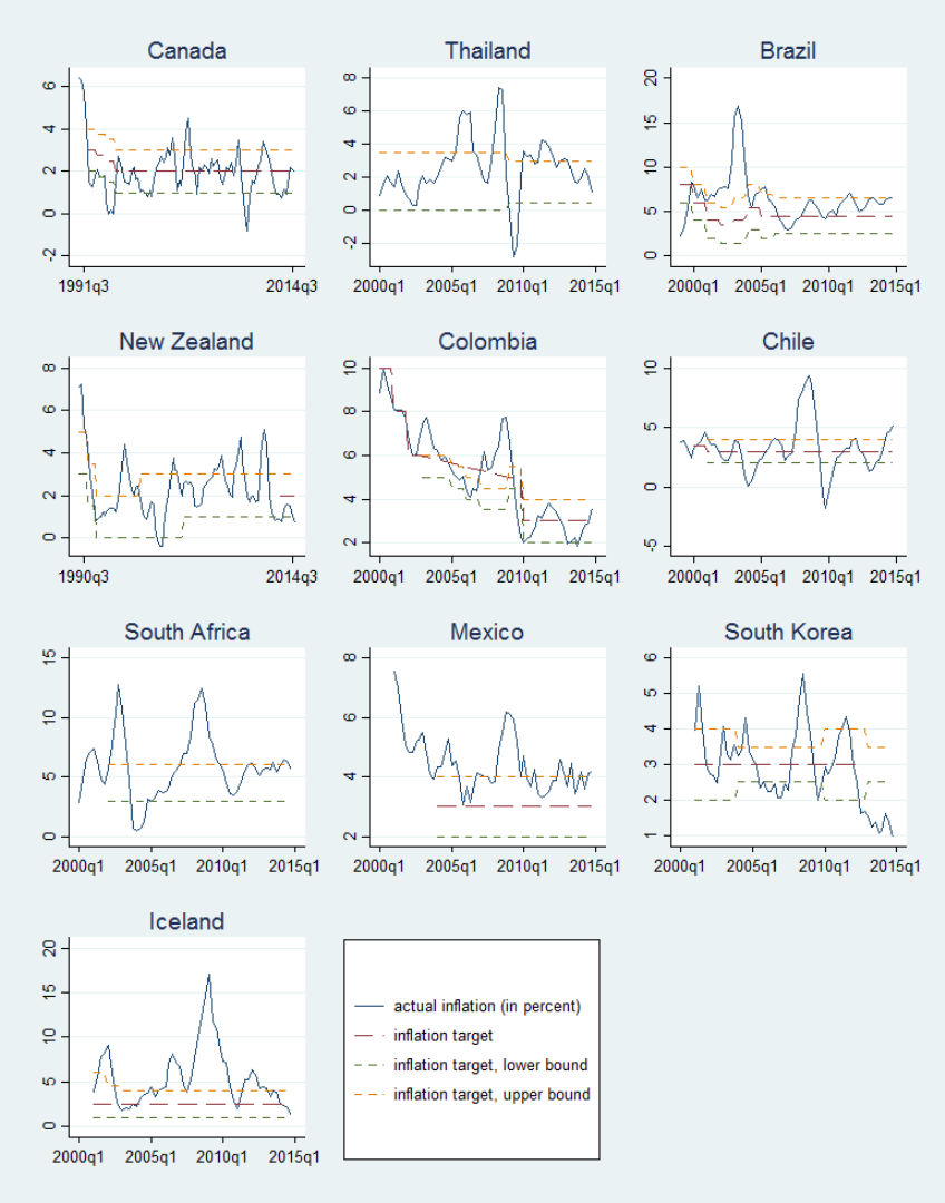
Figure 6: Performance of Inﬂation Targeting Countries: Top Group

Figure 7: Performance of Inﬂation Targeting Countries: Bottom Group

Table 6: Performance of Inﬂation Targeting Countries: Percent of Time Inﬂation

within the Announced Range

Top inﬂation targeters Bottom inﬂation targeters

Canada 70% Peru 44%

Thailand 65% Australia 40%

Brazil 64% Czech Republic 40%

New Zealand 61% Indonesia 38%

Colombia 60% Philippines 38%

Chile 57% Israel 35%

South Africa 50% Turkey 28%

Mexico 48% Poland 27%

South Korea 46% Serbia 18%

Iceland 46% Romania 18%

Results from Table 5 indicate that the assumption is well-grounded. For inﬂation

targeting countries, the results are more pronounced, compared to the baseline re-

sult. When only inﬂation targeting countries are considered, the estimated eﬀects

are larger and statistically more signiﬁcant. On average, real stock returns respond

more negatively to expected and unexpected inﬂation, and this is true in both ad-

vanced and emerging markets. When the interaction terms between inﬂation and

policy rate cyclicality are included, the estimated coeﬃcients are extremely negative

and statistically signiﬁcant for advanced markets, but not for emerging markets. This

may reﬂect the fact that the credibility of the central banks diﬀer in advanced and

emerging markets.

To understand why stock returns do not respond to monetary policy cyclicality in

emerging market inﬂation targeters, I further explore central banks’ track record of

controlling inﬂation by examining inﬂation performance with respect to central banks’

inﬂation target bands. While many central banks target medium-term inﬂation and

no central bank intends to keep inﬂation within the announced band at every point

in time, a persistent period of inﬂation falling outside the target band raises concerns

about a central bank’s capacity and credibility in controlling inﬂation. My approach

to classify inﬂation targeting countries is similar to the idea of coding countries by

their de facto exchange rate regime. To the extent of my knowledge, no academic

study has done such exercise before. Among the 30 inﬂation targeting countries in

the sample, 24 of them have more than 5 years of experience, and 20 of them have

Table 7: Regressions on Real Stock Returns by Monetary Policy Framework: Inﬂation Targeting, Continued.

Dependent variable: real stock return (1) (2) (3) (4) (5) (6) (7) (8) (9)

Expected inﬂation -2.506*** -3.743*** -2.066** -3.675*** -1.746 -3.645*** -0.984 -0.888 -0.548

(0.866) (0.865) (0.977) (0.935) (1.287) (0.942) (2.402) (5.557) (1.362)

Unexpected inﬂation -2.912*** -3.390*** -1.704 -3.882*** -0.541 -3.812*** 0.0113 5.859 -3.897**

(0.856) (0.591) (1.362) (0.755) (1.685) (1.326) (2.995) (4.990) (1.843)

Expected inﬂation × policy rate cyclicality 0.628 -4.278* -11.51** 0.385 -3.543 3.347 -25.13***

(1.379) (2.450) (4.539) (1.621) (8.354) (13.07) (5.278)

Unexpected inﬂation × policy rate cyclicality -1.550 -4.016 -10.18** -1.520 -7.596 3.035 -17.15**

(1.937) (2.581) (4.952) (1.750) (8.925) (14.12) (7.337)

Exp. inﬂation × countercyclical policy dummy -5.088** -0.181

(2.478) (1.087)

Une. inﬂation × countercyclical policy dummy -5.644* 0.0974

(3.237) (2.010)

Industrial production growth rate 1.085*** 1.140*** 1.218*** 0.987** 1.143*** 0.980** 1.455*** 1.302*** 1.449***

(0.275) (0.240) (0.188) (0.400) (0.194) (0.399) (0.261) (0.415) (0.464)

M2 growth rate -0.254 -0.430 -0.570 -0.237 -0.606 -0.232 0.224 -1.506*** -0.924

(0.217) (0.296) (0.479) (0.187) (0.512) (0.184) (0.258) (0.475) (0.566)

Improvement in ﬁnancial risk rating 0.0193*** 0.0172*** 0.0135** 0.0174* 0.0134* 0.0172* 0.0264*** 0.0436** -0.00714

(0.00572) (0.00504) (0.00656) (0.00968) (0.00719) (0.00969) (0.00652) (0.0207) (0.00666)

U.S 3-month Treasury bill yield rate 0.0109 0.0164 0.0204 0.00786 0.0216 0.00818 0.0187 -0.00126 0.0167

(0.0147) (0.0129) (0.0127) (0.0173) (0.0132) (0.0172) (0.0137) (0.0170) (0.0218)

VIX -0.0118*** -0.0125*** -0.00882*** -0.0171*** -0.00916*** -0.0170*** -0.00845*** -0.00395 -0.00856***

(0.00272) (0.00262) (0.00196) (0.00414) (0.00200) (0.00414) (0.00269) (0.00556) (0.00271)

Constant 0.408*** 0.470*** 0.424*** 0.511*** 0.439*** 0.512*** 0.241** 0.297** 0.590***

(0.0819) (0.0910) (0.0857) (0.104) (0.0932) (0.105) (0.110) (0.113) (0.112)

Sample Long-term all IT top IT bottom IT top IT bottom IT top IT top IT top IT

EM IT w/ band in band in band in band in band π within range π below range π above range

Observations 558 918 530 388 530 388 292 57 153

R-squared 0.3966 0.4287 0.4599 0.4544 0.4287 0.4537 0.3585 0.3994 0.6359

Number of countries 11 18 9 9 9 9 9 7 9

Note: Driscoll-Kraay standard errors in parentheses. *** p < 0.01; ** p < 0.05; * p < 0.1.

announced explicit inﬂation bands to the public. I divide these 20 countries into two

groups based on the percent of time inﬂation remains in the range announced by the

central bank (Figures 6 and 7).

The results are reported in Table 6 and they reveal

staggering diﬀerences in central banks’ tendency in managing inﬂation.

Canada

as the top performer keeps inﬂation within the target band for 70% of the time.

On the other hand, the central bank in Romania has faced overwhelming diﬃculties

in steering inﬂation towards their target band and as a result inﬂation is within

the announced range for only 18% of the period. The threshold is 45% to separate

the sample into top and bottom groups. Results in Column 1 of Table 7 shows

that emerging market inﬂation targeters with more than 10 years of experience in

general are not successful in shaping market perceptions. It is the history of inﬂation

targeting record rather than the length of the record that matters. Announcing the

inﬂation band helps a little bit in shaping market perceptions, as shown in Column

2. Furthermore, markets are reacting to monetary policy cyclicality in the top group,

but not so in the bottom group. This means that central banks’ ability to maintain

inﬂation within their target bans is key to shape market perceptions.

The inﬂation targeting countries in the top group, which include both advanced

and emerging markets, maintain inﬂation within their target bands most of the time,

and markets pay attention to monetary policy cyclicality. Instead, the inﬂation tar-

geting countries in the bottom group are struggling to keep inﬂation in the announced

bands. As a result, markets do not pay much attention to monetary policy cyclical-

ity.

In reality, this calculation is complicated by the fact that central banks use diﬀerent underlying

inﬂation measures (for example, headline CPI vs. core CPI), various target horizons (1 year or

mid-term), revisions in targets at certain points in time, and adjustments made by authorities to

account for structural breaks such as one-oﬀ tax changes. Nevertheless, given the nature of the

study, and the way countries are grouped into two categories, this approach illustrates the point of

central bank credibility and capability, and serves the purpose well.

It is worth noting idiosyncrasies in inﬂation targeting bands in diﬀerent countries. Certain

countries have set themselves more diﬃcult tasks due to tighter bands. For instance, Australia’s

inﬂation target band is 1 percentage point wide (2–3 percent), while Canada’s is 2 percentage points

wide (1–3 percent). If Australia’s target range had instead been a 2 percentage points, we would have

seen a higher share of the time within that range for Australia. Nevertheless, this paper adopts a

fact-based approach that only uses central banks’ oﬃcial inﬂation bands to assess inﬂation targeting

countries.

Ilzetzki, Reinhart and Rogoﬀ (2017) make a similar argument that inﬂation targeting countries

are heterogeneous and far less distinctive as one group than advertised. Using event studies and

estimating an augmented Taylor rule for the inﬂation targeting group, they show that inﬂation

targeting central banks diﬀer in the degree of stabilzing inﬂation and managing exchange rates.

Finally, for the top inﬂation targeters, I split the results by looking at scenarios

when inﬂation is within, below or above the target band. In these countries, when

inﬂation is outside the target band, it is three times more likely to see inﬂation is

above the band (153 observations in regression) than inﬂation is below the band (57

observations in regression). Regression results indicate that the interaction terms are

extremely signiﬁcant when inﬂation is above the range, but they are not signiﬁcant

when inﬂation is within or below the range. This echoes the fact that historically,

central banks are more concerned with inﬂation above the band and react asym-

metrically to inﬂation dynamics with respect to the target. For the top inﬂation

targeting countries with relative successful experience, markets learn from history

and are most sensitive when inﬂation is above the range, but are unresponsive when

inﬂation is within or below the range.

4.4 Results with Respect to the Zero Lower Bound (ZLB)

Lastly, I explore whether the stock return-inﬂation relation changes when mone-

tary policy is constrained by the Zero Lower Bound. The onset of the Global Finan-

cial Crisis (GFC) has prompted central banks around the world to lower their policy

rates, and policy rates in a number of countries have hit the Zero Lower Bound.

These countries include the United States, the Euro Area economies, Switzerland,

Japan and several others. A natural question to ask is whether real stock returns

still respond negatively to inﬂation, if the Zero Lower Bound is binding. To formally

analyze this question, I run the following regression:

i,t

= β

+β

i,t

(1−ZLB)+β

i,t

ZLB+β

i,t

(1−ZLB)+β

i,t

ZLB+ZΓ+u

+

i,t

(3)

here I use actual inﬂation in the regression and interact it with a ZLB dummy

variable. When ZLB=1, policy rate is hindered by the ZLB. A Zero Lower Bound

(ZLB) episode is identiﬁed if policy rate is below or equal to 25 basis points for a

given country. The conjecture for this regression is that real stock returns respond

asymmetrically to inﬂation and monetary policy cyclicality, depending on whether

policy rate hits the Zero Lower Bound or not, and real stock returns respond the

Table 8: Regressions on Real Stock Returns with Respect to the Zero Lower Bound (ZLB)

Dependent variable: real stock return (1) (2) (3) (4) (5) (6)

Inﬂation × (1- ZLB) -1.459*** -5.808*** -1.792*** -2.522*** -0.808*** -2.588

(0.339) (0.905) (0.313) (0.835) (0.251) (1.602)

Inﬂation × ZLB -1.431 -0.365 -3.027 5.699 -4.476* 8.354

(1.511) (2.174) (1.945) (7.864) (2.287) (9.471)

Inﬂation × (1- ZLB) × policy rate cyclicality -4.871*** -7.215***

(0.879) (1.734)

Inﬂation × ZLB × policy rate cyclicality 2.034 -13.09

(3.423) (11.36)

Inﬂation × (1- ZLB) × countercyclical policy dummy -4.044*** -3.472*

(0.659) (1.807)

Inﬂation × ZLB × countercyclical policy dummy 3.601 -8.990

(3.099) (10.28)

Industrial production growth rate 1.178*** 0.905*** 1.215*** 0.961*** 1.220*** 0.914***

(0.166) (0.183) (0.170) (0.182) (0.164) (0.187)

M2 growth rate 0.383** -0.0220 0.406** 0.00554 0.386** -0.00864

(0.186) (0.289) (0.193) (0.275) (0.194) (0.288)

Improvement in ﬁnancial risk rating 0.0132*** 0.000739 0.0122** 0.000924 0.0117** 0.000793

(0.00502) (0.00573) (0.00497) (0.00559) (0.00490) (0.00582)

U.S 3-month Treasury bill yield rate 0.00453 0.0220** 0.00947 0.0211** 0.0105 0.0221**

(0.0108) (0.0109) (0.0106) (0.0104) (0.0103) (0.0108)

VIX -0.0169*** -0.0165*** -0.0163*** -0.0166*** -0.0161*** -0.0167***

(0.00316) (0.00273) (0.00293) (0.00269) (0.00293) (0.00272)

Constant 0.360*** 0.415*** 0.376*** 0.426*** 0.375*** 0.417***

(0.0809) (0.0723) (0.0756) (0.0703) (0.0741) (0.0721)

Sample full AM full AM full EM

Observations 3,663 1,945 3,498 1,944 3,498 1,944

R-squared 0.3708 0.4484 0.4002 0.4587 0.4036 0.4512

Number of countries 57 27 55 27 55 27

Note: Driscoll-Kraay standard errors in parentheses. *** p < 0.01; ** p < 0.05; * p < 0.1.

same to other control variables.

By comparing stock market reactions under normal times and the Zero Lower

Bound periods, we ﬁnd an interesting phenomenon (Table 8). In normal times, when

the Zero Lower Bound does not bind, we observe the conventional relationship: real

stock returns respond negatively to inﬂation, and stock returns react more negatively

to inﬂation when monetary policy becomes more countercyclical. For the periods

when monetary policy is restricted by the ZLB, the estimated coeﬃcients on inﬂation,

and the interaction terms between inﬂation and monetary policy cyclicality measures

are no longer signiﬁcant. This means we cannot reject that real stock returns do not

respond to inﬂation and monetary policy cyclicality under ZLB episodes. When it

comes to inﬂation dynamics, stock markets seem to perceive the Zero Lower Bound as

a diﬀerent regime. The fact that inﬂation is usually low under the Zero Lower Bound

indicates that a positive inﬂation surprise is good news, because the real interest

rate is lower and the central bank does not need to respond to the upside inﬂation

development. If there is a negative inﬂation surprise, there will be additional costs if

the central bank decreases the policy rate and policymakers may be more reluctant to

lower the rate. In addition, a possible Eﬀective Lower Bound (ELB), where the central

bank can no longer decrease its policy rate to stimulate the economy, is potentially

noted by markets as well.

Nevertheless, since the Zero Lower Bound is a new phenomenon for most countries,

the limited number of observations and low statistical power suggests that the readers

need to interpret the results with caution. Indeed, the standard errors are much

larger under the Zero Lower Bound episodes. The analysis here primarily focuses on

advanced markets since there are very few Zero Lower Bound episodes for emerging

markets.

5 Robustness Check

I have done the following robustness checks: re-run the augmented regression using

actual inﬂation and test whether the stock return-inﬂation relation is less negative in

Only three emerging markets in Eastern Europe (Bulgaria, Latvia and Lithuania.) have hit the

Zero Lower Bound in recent years.

emerging markets. A dummy variable for emerging market is interacted with actual

inﬂation, and the interaction term is positive and statistically signiﬁcant; drop the ob-

servations when countries adopted the Euro. When countries join the Eurozone, they

lose monetary autonomy. Excluding such observations in a currency union allows us

to investigate market reactions to domestic monetary policy; exclude hyperinﬂation

periods. Drop observations with inﬂation higher 50% or 100% in the regression; use

Consensus Forecasts data as measures of expected inﬂation; construct a global stock

return factor by aggregating stock returns in Systemic-5 countries (United States,

United Kingdom, Germany, Japan and China, weighted by nominal GDP) and in-

clude it as a control variable. The global factor is statistically signiﬁcant, which

means that stock returns in systemic countries is highly correlated with domestic

market performance; replace the U.S. Treasury bill yield with Wu-Xia shadow federal

funds rate to account for the issue of unconventional monetary policy at the Zero

Lower Bound in the United States. The results remain mostly the same and they are

reported in the appendix.

There are several limitations in this paper. First, the monetary policy cyclicality

measure is computed as a constant throughout the sample period for a given coun-

try. Since monetary policy cyclicality could vary over time, this is a coarse measure.

Results may be aﬀected, especially when dividing countries by monetary policy frame-

work, which is evolving as well. One potential improvement is to make policy rate

cyclicality time-varying by decade.

The second caveat is regarding the inﬂation expectation measure. This paper de-

ﬁnes inﬂation expectation based on forecasts from surveys or models. Conceptually,

inﬂation forecast is not exactly the same as inﬂation expectation. However, because

inﬂation expectations are not known in general, the inﬂation forecasts are the best

measures available for many countries for a long period of time. Market-based mea-

sures of inﬂation expectations, such as estimates of inﬂation compensation embedded

in the returns of ﬁnancial instruments, are only available for a limited set of countries

in recent years.

Lastly, the issue of cross-border listings and multinational ﬁrms blurs the bound-

aries of national stock returns. For example, a Chinese company chooses its Initial

Public Oﬀering (IPO) in Nasdaq runs most of its businesses outside the U.S., or a

multinational corporation listed in the New York Stock Exchange receives most of its

revenues from abroad. When such companies are included as component stocks,

the underlying indices no longer perfectly represent national economic activities.

Given these cases happen primarily in advanced countries and this paper studies

71 economies, the problem will not change the results substantially or qualitatively.

6 Discussion and Conclusion

As major central banks are conducting reviews on monetary policy frameworks

and tools, this paper ﬁnds that how a central bank reacts to inﬂation plays a critical

role in determining the stock return-inﬂation relation. In August 2020, the Federal

Reserve announced a revision to its monetary policy framework by setting an Average

Inﬂation Target (AIT) of 2 percent over the long-run, allowing for a period of above-

the-target inﬂation to oﬀset low inﬂation in the past decade. The European Central

Bank has replaced its inﬂation target of below but close to 2 percent with a symmetric

target of 2 percent over the medium term. These changes will have implications on

the stock return-inﬂation relation in the future.

This paper contributes to the stock return-inﬂation literature by examining how

monetary policy shapes the stock return-inﬂation relation using a novel dataset of

71 advanced and emerging markets. The empirical results support the view that the

stock return–inﬂation relation is partially driven by monetary policy cyclicality. If

a country’s central bank pursues a more countercyclical monetary policy, the stock

return-inﬂation relation becomes more negative. The results highlight how the market

anticipates monetary policy under a variety of regimes with implications for policy

under exchange rate pegs, inﬂation targeting and the Zero Lower Bound (Figure 8).

Results suggest that central banks’ decisions on policy cyclicality and the instru-

ments employed in the toolkit not only aﬀect real economic activities, but also result

in a shift in the response of stock prices to inﬂation developments. Although the

issue of whether monetary policy should respond to asset prices is still under debate,

stock price ﬂuctuations, especially the ones caused by monetary policy, deserve atten-

tion. In advanced markets, the Global Financial Crisis has prompted major central

banks lowered their policy rates to the Zero Lower Bound and expanded asset pur-

chase programs. The fact that the policy rates are constrained by their lower bounds

Figure 8: Summary of Main Findings

has resulted in changing patterns of stock return-inﬂation relations in those coun-

tries. This is because central banks can no longer lower policy rates when inﬂation

decreases, but can still raise policy rates as usual when inﬂation increases. Gourio

and Ngo (2016) document a structural break in the response of stock prices to inﬂa-

tion in the United States after 2008. In emerging markets, policymakers should pay

special attention to rapid expansions in monetary aggregate, since they can create

bubbles in the stock prices and pose a threat to ﬁnancial stability. Results also imply

that central banks that are on market surveillance can do more to shape the mar-

ket perception of inﬂation shocks than simply monitor the stock market movements.

Central banks’ communication to the market is a key to success and the eﬀectiveness

of such communications critically depends on central banks’ credibility. Speciﬁcally,

central banks can commit to more countercyclical monetary policy to change the way

stock market reacts to inﬂation. This is particularly relevant, given that a number of

emerging markets have evolved from procyclical to countercyclical monetary policy

over the last decade (Vegh and Vuletin, 2012).

Results also indicate that practitioners and policymakers in emerging markets

should use caution when borrowing the experience from advanced markets. The stock

return-inﬂation relations are distinct in advanced and emerging markets because of

diﬀerences in the monetary policy cyclicality, the underlying monetary policy frame-

work, central bank’s capacity and credibility, and whether policy rate is conﬁned by

the Zero Lower Bound. Countries’ monetary policy frameworks vary signiﬁcantly as

central banks target diﬀerent nominal anchors: exchange rate, inﬂation, monetary

aggregate or others. Policy rate cyclicality is the main monetary policy factor that

aﬀects the stock return-inﬂation relation in both advanced and emerging markets,

while monetary aggregate growth is also relevant in emerging markets.

There are several possible areas for future research: First, one can further examine

the relationship with respect to business cycle conditions. Does the result change

during moderate or signiﬁcant expansions and contractions? Do the amplitude and

duration of the business cycles aﬀect the results? What is the interaction between the

real business cycles and the ﬁnancial cycles? Fama and French (1989) argue that the

expected returns on stocks and bonds are lower when economic conditions are strong

and higher when conditions are weak. Wei (2009) ﬁnds that the U.S. nominal equity

returns respond more negatively to unexpected inﬂation during economic contractions

than expansions. Harding and Pagan (2002) propose an algorithm to locate turning

points in the natural logarithm of a series, and their methodology is extensively

adopted to deﬁne and measure business cycles. Several researchers (Claessens et al.,

2011; Drehmann et al., 2012) have identiﬁed economic and ﬁnancial cycles based on

the approach.

Second, the study can be extended to several open economy and institutional

angles. Many emerging markets are typical small open economies and sensitive to ex-

ternal conditions. It will be interesting to study the role of exchange rate movements

and capital ﬂows. Particularly, one can investigate problems that are largely associ-

ated with emerging markets. For example, do results diﬀer by crisis types? Are the

diﬀerences of the stock return-inﬂation relation among countries due to institutional

quality, the stock market openings to foreign investors (Kim and Singal, 2000), or

ﬁnancial liberalization (Kaminsky and Schmukler, 2008)?

Third, this paper conﬁrms that there exists a negative relationship between real

stock returns and inﬂation at the quarterly horizon for many countries. However, it

is also useful to examine how stock prices react to inﬂation at long horizons. Previous

research (Boudoukh and Richardson, 1993; Harrison and Zhang, 1999; Schotman and

Schweitzer, 2000; Kim and In, 2005) has found a positive relationship between stock

returns and inﬂation over long horizons, and results support the Fisher hypothesis as

the horizon increases.

References

Adrian, Tobias, Shin, Hyun Song, 2010, “The Changing Nature of Financial In-

termediation and the Financial Crisis of 2007–2009”, Annual Review of Economics,

Vol.2:1-698.

Baker, Malcolm, Stein, Jeremy C. and Wurgler, Jeﬀrey, 2003, ”When Does The

Market Matter? Stock Prices And The Investment Of Equity-Dependent Firms,”

Quarterly Journal of Economics, v118, 969-1006.

Bakshi, G. S. and Chen, Z., 1996, “Inﬂation, asset prices, and the term structure

of interest rates in monetary economics”, Review of Financial Studies, 9, 241-275.

Boudoukh, Jacob and Richardson, Matthew, 1993, ”Stock Returns and Inﬂation:

A Long-Horizon Perspective”, The American Economic Review, Vol. 83, No. 5, pp.

1346-1355.

Boyle, Glenn W. and Peterson, James D., 1995, ”Monetary Policy, Aggregate

Uncertainty, and the Stock Market”, Journal of Money, Credit and Banking, Vol. 27,

No. 2, pp. 570-582.

Brandt, M. and Wang, K., 2003, “Time-varying risk aversion and unexpected

inﬂation”, Journal of Monetary Economics, 50, 1457-1498.

Campbell, J. and Vuolteenaho, T., 2004, “Inﬂation Illusion and Stock Prices”,

American Economic Review, 94, 19-23.

Chen, Nai-Fu, Roll, Richard and Ross, Stephen A., 1986, ”Economic Forces and

the Stock Market”, The Journal of Business, Vol. 59, No. 3, pp. 383-403.

Chen, S., 2007, “Does Monetary Policy Have Asymmetric Eﬀects on Stock Re-

turns?”, Journal of Money, Credit and Banking, Vol.39, No. 2-3.

Chinn, Menzie D. and Ito, Hiro, 2006, ”What Matters for Financial Development?

Capital Controls, Institutions, and Interactions,” Journal of Development Economics,

Volume 81, Issue 1, Pages 163-192.

Christiano, Lawrence, Ilut, Cosmin, Motto, Roberto, Rostagno, Massimo, 2010.

”Monetary policy and stock market booms,” Proceedings - Economic Policy Sympo-

sium - Jackson Hole, Federal Reserve Bank of Kansas City, pages 85-145.

Claessens, Stijn , Kose, M. Ayhan and Terrones, Marco E., 2011, ”Financial

Cycles: What? How? When?” IMF Working Paper 11/76.

Cubeddu et al., 2014, “Emerging Markets in Transition: Growth Prospects and

Challenges”, IMF Staﬀ Discussion Note 14/06.

Drehmann, Mathias, Borio, Claudio and Tsatsaronis, Kostas, 2012, ”Character-

ising the ﬁnancial cycle: don’t lose sight of the medium term!”, BIS Working Papers

No 380.

Driscoll, J., and Kraay, A., 1998, “Consistent covariance matrix estimation with

spatially dependent panel data,” The Review of Economics and Statistics, 80(4),

549–560.

Erb, CB, Harvey, CR , Viskanta, TE, 1995, ”Inﬂation and world equity selection”,

Financial Analysts Journal, Volume 51 Issue 6.

Fama, E., 1981. “Stock returns, real activity, inﬂation, and money”, American

Economic Review, 71, 545–65.

Fama, E. and Schwert, W., 1977, “Asset returns and inﬂation”, Journal of Finan-

cial Economics, 5, 115–46.

Fama, E. and French, K., 1989, “Business Conditions and Expected Returns on

Stocks and Bonds”, Journal of Financial Economics, 25, 23-49.

Feldstein, M., 1980, “Inﬂation and the Stock Market”, American Economic Re-

view, 70 (5), 839-847.

Geske, R. , Roll, R., 1983, ”The ﬁscal and monetary linkage between stock returns

and inﬂation”, the Journal of Finance, Volume 38, Issue 1, Pages 1–33.

Gourio, Francois, Ngo, Phuong, 2016, ”Risk Premia at the ZLB: a macroeconomic

interpretation”, working paper.

Gultekin, NB, 1983, ”Stock market returns and inﬂation: evidence from other

countries”, Journal of Finance, Vol. 38, No. 1, pp. 49-65.

Harding, D. and Pagan, A., 2002. “Dissecting the cycle: a methodological inves-

tigation”, Journal of Monetary Economics, 365-381.

Harrison, Paul and Zhang, Harold H., 1999, ”An Investigation of the Risk and

Return Relation at Long Horizons”, Vol. 81, No. 3, Pages 399-408.

Hoechle, D., 2007, “Robust standard errors for panel regressions with cross-

sectional dependence,” The Stata Journal, 7(3), 281–312.

Ilzetzki, Ethan, Reinhart, Carmen M., Rogoﬀ, Kenneth S., 2017, ”Exchange Ar-

rangements Entering the 21st Century: Which Anchor Will Hold?”, NBER Working

Paper No. 23134.

Kaminsky, Graciela L., Carmen M. Reinhart, and Carlos A. Vegh, 2005, “When

It Rains, It Pours: Procyclical Capital Flows and Macroeconomic Policies,” in NBER

Macroeconomics Annual 2004, Vol.19, ed. by Mark Gertler and Kenneth Rogoﬀ.

Kaminsky, G. and Schmukler, S., 2008, ”Short-Run Pain, Long-Run Gain: Finan-

cial Liberalization and Stock Market Cycles,” Review of Finance, Oxford University

Press for European Finance Association, vol. 12(2), pages 253-292.

Katz, Michael, Lustig, Hanno, Nielsen, Lars , 2017, ”Are Stocks Real Assets?

Sticky Discount Rates in Stock Markets”, Review of Financial Studies, (2017) 30 (2):

539-587.

Kaul, G., 1987 ”Stock returns and inﬂation: The role of the monetary sector”,

Journal of Financial Economics, 18 253-276.

Kim, Sangbae and In, Francis, 2005, ”The relationship between stock returns and

inﬂation: new evidence from wavelet analysis”, Journal of Empirical Finance, Volume

12, Issue 3, Pages 435–444.

Kim, E. Han, Singal, Vijay, 2000, “Stock Market Openings: Experience of Emerg-

ing Economies”, Journal of Business, vol. 73, no.1.

Lintner, J., 1975, “Inﬂation and security returns”, Journal of Finance, 30, 259-280.

Marshall, D., 1992, ”Inﬂation and Asset Returns in a Monetary Economy”, Jour-

nal of Finance, Volume 47, Issue 4, Pages 1315–1342.

Modigliani, F. and Cohn, R. 1979, “Inﬂation, Rational Valuation, and the Mar-

ket”, Financial Analyst Journal, 35, 24-44.

Outreville, J. F., 2015, “The relationship between relative risk aversion and the

level of education: a survey and implications for the demand for life insurance”,

Journal of Economic Surveys, Volume 29, Issue 1, Pages 97–111.

Pastor, Lubos, and Veronesi, Pietro, 2003, ”Stock Prices and IPO Waves”, NBER

Working Paper No. 9858. Schmeling, Maik, 2009, ”Investor sentiment and stock

returns: Some international evidence ”, Journal of Empirical Finance, Volume 16,

Issue 3, Pages 394–408.

Schmeling, Maik, and Schrimpf, Andreas, 2011. ”Expected inﬂation, expected

stock returns, and money illusion: What can we learn from survey expectations”,

European Economic Review, 55 702–719.

Schotman, Peter C. and Schweitzer, Mark, 2000, ”Horizon sensitivity of the in-

ﬂation hedge of stocks”, Journal of Empirical Finance, Volume 7, Issues 3–4, Pages

301–315.

Sellin, P. , 2001, “”Monetary policy and the stock market: theory and empirical

evidence””, Journal of Economic Surveys, Volume 15, Issue 4, Pages 491–541.

Spyrou, SI, 2004, “Are stocks a good hedge against inﬂation? Evidence from

emerging markets”, Applied Economics, 41-48.

Vegh, Carlos A. and Guillermo Vuletin, 2012, “Overcoming the Fear of Free

Falling: Monetary Policy Graduation in Emerging Markets,” NBER Working Paper

No. 18175. Wei, Chao, 2009. “Does the stock market react to unexpected inﬂation

diﬀerently across the business cycle”, Applied Financial Economics, 1947-1959.

Wu, Jing Cynthia, and Xia, Fan Dora, 2014, “Measuring the Macroeconomic

Impact of Monetary Policy at the Zero Lower Bound”, NBER Working Paper No.

20117, May 2014.

Appendix

Data Description

Quarterly data from 1980Q1 to 2015Q2. The sample includes 71 economies, cov-

ering both advanced and emerging markets.

Country Classiﬁcation by Income Group

Advanced Markets (33): Australia, Austria, Belgium, Canada, Cyprus, Czech

Republic, Denmark, Estonia, Finland, France, Germany, Greece, Hong Kong SAR,

Iceland, Ireland, Israel, Italy, Japan, Luxembourg, Malta, Netherlands, New Zealand,

Norway, Portugal, Singapore, Slovak Republic, Slovenia, South Korea, Spain, Sweden,

Switzerland, United Kingdom, United States.

Emerging Markets (38): Argentina, Bosnia and Herzegovina, Brazil, Bulgaria,

Chile, China, Colombia, Costa Rica, Croatia, Egypt, Hungary, India, Indonesia, Ja-

maica, Jordan, Kazakhstan, Latvia, Lebanon, Lithuania, Macedonia, Malaysia, Mex-

ico, Morocco, Pakistan, Panama, Peru, Philippines, Poland, Romania, Russia, Serbia,

South Africa, Sri Lanka, Thailand, Tunisia, Turkey, Ukraine, Venezuela.

Note: the country classiﬁcation is based on the International Monetary Fund

(IMF)’s World Economic Outlook (WEO).

Panel Data Tests

Unit root tests are based on Augmented Dickey–Fuller, DF-GLS and Phillips–Perron

tests on each variable by country, as well as Im-Pesaran-Shin and Fisher-type tests.

Given the panel data is unbalanced in nature, several panel unit root tests are not

applicable. Detailed results are available upon request.

Tests for cross-sectional dependence cannot be performed. Given the nature of

the dataset, assume cross-section dependence and spatial eﬀects exist.

Wooldridge test for autocorrelation in panel data: we reject the null hypothesis

and conclude that the data does have ﬁrst-order autocorrelation.

Modiﬁed Wald test for groupwise heteroscedasticity in ﬁxed eﬀect regression model:

we reject the null hypothesis and conclude that the data has heteroscedasticity.

Table 9: Variable Description

Symbol Deﬁnition Data source/ Transformation

Original series

stock index Stock market index Bloomberg

RGDP Real GDP Haver Analytics, IMF IFS and WEO databases.

CPI Consumer price index IMF INS database

inﬂation CF current Inﬂation forecasts, current year Consensus Forecasts

inﬂation CF next Inﬂation forecasts, next year Consensus Forecasts

IP Industrial Production Datastream and IMF IFS databases

M2 M2 (money supply) Haver Analytics and IMF IFS databases

ﬁnancial risk ICRG ﬁnancial risk ratings, International Country Risk Guide (ICRG) database

from a high of 50 (least risk) to a low of 0 (highest risk).

TB3MS U.S. three-month Treasury Bill: Secondary Market Rate Board of Governors of the Federal Reserve System

VIX VIX Bloomberg

PR Central bank’s policy rate Haver Analytics, IMF IFS and GDS databases.

WuXiaShadowRate Wu-Xia shadow federal funds rate Federal Reserve Bank of Atlanta

MPF Monetary policy framework AREAER database, IMF.

inﬂation

target Inﬂation targets Central banks’ websites

inﬂation target lower Inﬂation bands, lower bounds. Central banks’ websites

inﬂation target upper Inﬂation bands, lower bounds. Central banks’ websites

Derived series

stock returny Nominal stock return (log) ln[stock index(t)] – ln[stock index(t-4)]

real stock index Real stock market index stock index/ CPI

real stock returny Real stock return (log) ln[real stock index(t)] – ln[real stock index(t-4)]

inﬂationy Inﬂation (log) ln[CPI(t)] – ln[CPI(t-4)]

inﬂationy e Expected inﬂation The measure based on the best forecasting accuracy:

predicted inﬂation from AR(4) model

inﬂationy u Unexpected inﬂation Actual inﬂation – expected inﬂation

IP growthy Industrial production growth ln[IP(t)] – ln[IP(t-4)]

M2 growthy Monetary aggregate growth ln[M2(t)] – ln[M2(t-4)]

ﬁnancial risk change Improvement in ﬁnancial risk rating ﬁnancial risk(t) - ﬁnancial risk (t-1)

MP correlation PR Policy rate cyclicality Correlation between the cyclical

components of real output and policy rate.

G5 real stock returny Systemic-5 real stock return Weighted average of real stock returny

in the US, UK, Germany, Japan and China.

Additional Tests on the Role of Monetary Policy

In a seminal paper, Bakshi and Chen (1996) oﬀer a tractable asset pricing model in

a monetary economy. In the representative-agent economy, the price level, inﬂation,

asset prices, the nominal and real interest rates are determined simultaneously and

in relation to each other. The inﬁnitely lived agent chooses consumption, money

demand, and portfolio holdings at each point of time to maximize expected life utility.

Monetary policy in this economy is such that the resulting money supply follows a

stochastic process over time. Based on a Money in the Utility Function Model (MIUF)

and an economy with i.i.d. output and money growth processes, the authors show

that

cov

(

) = cov

(

) − var

(

) (4)

That is, the covariance between the real rate of return on equity and inﬂation

is equal to the covariance between real output growth and nominal money growth,

minus the variance of real output growth. In Fama’s (1981) proxy hypothesis, money

stock is considered as given. This implies a zero covariance between real output

and money, and therefore the covariance between real equity return and inﬂation is

negative. In Geske and Roll (1983), monetary policy (money) is countercyclical, thus

the covariance between real equity return and inﬂation is negative as well. Note that

the covariance can be positive if the ﬁrst term on the right hand side of the equation

dominates the second term. This is the case in Kaul (1987), where the relationship

between stock return and inﬂation is positive if the monetary authority conducts a

procyclical monetary policy.

Boyle and Peterson (1995) extend the theoretical framework of monetary policy

and stock returns to address the question of whether monetary policy matters, as

diﬀerent from the question whether money matters. They achieve this by assuming

that the monetary policy targets the growth rate of money.

In a Cash-in-Advance

(CIA) Model, the simpliﬁed reaction function of the monetary authority is given by:

= kλ



(5)

In the original version of the reaction function of Boyle and Peterson (1995), there is an additional

disturbance term θ which represents imperfect implementation of monetary policy.

where k > 0 is a constant and  is the elasticity of the monetary response to

an output shock. Under the assumption that λ

is i.i.d. and constant risk aversion

preferences, a central ﬁnding in Boyle and Peterson (1995) is the following relation:

cov

(lnq

∗

, lnΠ

) = cov(λ

, ( − 1)lnλ

) = ( − 1)var(λ

) (6)

where q

∗

= q

t−1

= y

t−1

, Π

= P

t−1

. Therefore, equity returns are neg-

atively correlated with inﬂation when monetary policy is countercyclical ( < 0) or

weakly procyclical (0 <  < 1), and the correlation is positive when monetary policy

is strongly procyclical ( > 1).

Linear Regression Model:

cov

(r, pi) = α + β

cov

(y, m) + β

var

(y) + 

(7)

Joint test: α = 0, β

= 1, β

= −1.

Table 10: Summary Statistics to Test the Bakshi-Chen Hypothesis

Variable Observation Mean Std. dev. Min Max

Cov(r, pi) 63 0.0179 0.1497 -0.0176 1.186

Cov(y, m) 63 0.0017 0.0030 -0.0023 0.015

Var(y) 63 0.0015 0.0016 0.00003 0.0075

To test whether the relationship between stock returns and inﬂation is partially

driven by monetary policy cyclicality, I test Equation (4), which is a simple rela-

tionship on two covariance terms and one variance term. There are 63 countries in-

cluded in the test, with diﬀerent sample periods, depending on data availability. The

cross-sectional regression utilizes a single observation from each country. Summary

statistics show that the covariance between real stock return and inﬂation is much

larger in terms of magnitude compared to the covariance between real output and

monetary aggregate, and the variance of real output. Results from Ordinary Least

Squares indicate that the covariance between the real rate of return on equity and

inﬂation is signiﬁcantly positively correlated with the covariance between real output

growth and nominal money growth and negatively correlated with the variance of real

output growth. The signs of the estimated coeﬃcients are pointing to the correct di-

Table 11: Test the Bakshi-Chen Monetary Policy Hypothesis

Dependent variable: cov(r, pi) (1) (2) (3) (4) (5) (6)

cov(y, m) 48.33** 48.27** -0.134 0.00199 50.65** 51.39**

(20.77) (21.34) (1.028) (0.904) (21.29) (21.51)

var(y) -58.47** -50.33** -0.659 -0.974** -62.55** -57.54**

(26.21) (23.12) (0.682) (0.446) (27.79) (25.85)

Constant 0.0254* -0.000381 0.0228

(0.0148) (0.000376) (0.0241)

Estimation method OLS OLS OLS OLS OLS OLS

Sample full full AM AM EM EM

Observations 63 63 32 32 31 31

R-squared 0.592 0.583 0.115 0.314 0.610 0.617

Note: Robust standard errors in parentheses. *** p < 0.01; ** p < 0.05; * p < 0.1.

rection, however, the relation suggested that the theory does not hold precisely, since

the estimated coeﬃcients are much bigger than 1 and -1, implied by Equation (4).

The estimated coeﬃcients for advanced markets are closer to theoretical predictions,

but the estimated coeﬃcients for emerging markets are far beyond theoretical predic-

tions. The unrealistic assumption of i.i.d. output and money growth processes makes

it diﬃcult to reconcile the discrepancy between theoretical predictions and empirical

ﬁndings.

Table 12: Robustness Check: Use Actual Inﬂation and Test the Stock Return-Inﬂation Relation is Less Negative in EMs

Dependent variable: real stock return (1) (2) (3) (4) (5) (6) (7) (8)

Inﬂation -1.785*** -2.200** -1.312*** -4.553*** -0.807*** -2.391 -0.863*** -3.637***

(0.313) (0.963) (0.274) (0.994) (0.250) (1.540) (0.260) (1.268)

Inﬂation × EM dummy 3.202*** 2.846**

(0.945) (1.201)

Inﬂation × policy rate cyclicality -4.851*** -7.553*** -2.172** -2.869***

(0.878) (1.750) (0.970) (0.714)

Inﬂation × countercyclical policy dummy -3.978*** -3.503** -2.255*** -2.416***

(0.677) (1.737) (0.676) (0.649)

Industrial production growth rate 1.218*** 0.973*** 1.434*** 1.240*** 1.223*** 0.926*** 1.446*** 1.239***

(0.169) (0.182) (0.227) (0.174) (0.162) (0.186) (0.218) (0.169)

M2 growth rate 0.410** 0.0197 0.634*** 0.404** 0.392** 0.00262 0.621*** 0.394**

(0.195) (0.279) (0.172) (0.194) (0.196) (0.293) (0.169) (0.195)

Improvement in ﬁnancial risk rating 0.0121** 0.00116 0.0212*** 0.0118** 0.0117** 0.000963 0.0209*** 0.0116**

(0.00498) (0.00569) (0.00520) (0.00494) (0.00492) (0.00587) (0.00509) (0.00492)

U.S 3-month Treasury bill yield rate 0.00880 0.0194* -0.00203 0.0104 0.00968 0.0200* -0.00150 0.0106

(0.0104) (0.0100) (0.0131) (0.0103) (0.0101) (0.0104) (0.0128) (0.0102)

VIX -0.0164*** -0.0168*** -0.0154*** -0.0161*** -0.0162*** -0.0169*** -0.0151*** -0.0161***

(0.00291) (0.00267) (0.00344) (0.00285) (0.00291) (0.00272) (0.00343) (0.00286)

Constant 0.379*** 0.432*** 0.310*** 0.380*** 0.377*** 0.424*** 0.310*** 0.378***

(0.0745) (0.0691) (0.0812) (0.0732) (0.0733) (0.0707) (0.0794) (0.0730)

Sample full AM EM full full AM EM full

Observations 3,498 1,944 1,554 3,498 3,498 1,944 1,554 3,498

R-squared 0.3992 0.455 0.3928 0.4078 0.4019 0.4468 0.3958 0.4076

Number of countries 55 27 28 55 55 27 28 55

Note: Driscoll-Kraay standard errors in parentheses. *** p < 0.01; ** p < 0.05; * p < 0.1.

Table 13: Robustness Check: Drop the Observations when Countries Adopted the Euro

Dependent variable: real stock return (1) (2) (3) (4) (5) (6)

Expected inﬂation -1.834*** -2.525** -1.341*** -0.791*** -3.120** -0.865***

(0.381) (1.012) (0.301) (0.289) (1.400) (0.292)

Unexpected inﬂation -1.627*** -1.017 -1.224*** -0.906 -3.264* -0.864*

(0.533) (1.985) (0.463) (0.596) (1.807) (0.517)

Expected inﬂation × policy rate cyclicality -5.205*** -10.69*** -2.362**

(1.093) (3.948) (1.052)

Unexpected inﬂation × policy rate cyclicality -2.746 -7.238* -0.951

(1.823) (4.196) (1.406)

Expected inﬂation × countercyclical policy dummy -4.372*** -4.354** -2.311***

(0.718) (1.748) (0.735)

Unexpected inﬂation × countercyclical policy dummy -2.885** 0.256 -2.241**

(1.142) (1.870) (0.949)

Industrial production growth rate 1.227*** 0.856*** 1.428*** 1.236*** 0.755*** 1.444***

(0.186) (0.229) (0.229) (0.178) (0.241) (0.221)

M2 growth rate 0.388* -0.334 0.638*** 0.371* -0.349 0.628***

(0.207) (0.335) (0.173) (0.206) (0.349) (0.170)

Improvement in ﬁnancial risk rating 0.0160*** 0.00438 0.0210*** 0.0156*** 0.00472 0.0208***

(0.00526) (0.00560) (0.00538) (0.00517) (0.00593) (0.00528)

U.S 3-month Treasury bill yield rate 0.00502 0.0150 -0.00203 0.00593 0.0157 -0.00168

(0.0106) (0.0101) (0.0131) (0.0103) (0.0106) (0.0128)

VIX -0.0152*** -0.0140*** -0.0153*** -0.0149*** -0.0141*** -0.0151***

(0.00294) (0.00227) (0.00345) (0.00293) (0.00233) (0.00345)

Constant 0.371*** 0.453*** 0.310*** 0.371*** 0.455*** 0.311***

(0.0802) (0.0672) (0.0810) (0.0775) (0.0701) (0.0793)

Sample full AM EM full AM EM

Observations 2,701 1,149 1,552 2,701 1,149 1,552

R-squared 0.3774 0.4564 0.3935 0.3825 0.443 0.3963

Number of countries 45 17 28 45 17 28

Note: Driscoll-Kraay standard errors in parentheses. *** p < 0.01; ** p < 0.05; * p < 0.1.

Table 14: Robustness Check: Drop Inﬂation Above 100%

Dependent variable: real stock return (1) (2) (3) (4) (5) (6)

Expected inﬂation -1.871*** -2.561** -1.355*** -0.929*** -2.498 -1.008***

(0.344) (0.990) (0.305) (0.273) (1.558) (0.281)

Unexpected inﬂation -1.347** -2.399 -1.305*** -1.162* -3.096 -1.074*

(0.573) (1.657) (0.474) (0.674) (2.127) (0.554)

Expected inﬂation × policy rate cyclicality -5.541*** -8.284*** -1.869*

(0.927) (1.704) (1.114)

Unexpected inﬂation × policy rate cyclicality -0.379 2.390 -0.305

(1.445) (2.687) (1.425)

Expected inﬂation × countercyclical policy dummy -4.327*** -4.387** -2.137***

(0.679) (1.768) (0.726)

Unexpected inﬂation × countercyclical policy dummy -1.134 2.615 -1.983**

(0.871) (2.063) (0.950)

Industrial production growth rate 1.180*** 0.872*** 1.435*** 1.189*** 0.818*** 1.452***

(0.165) (0.185) (0.230) (0.159) (0.192) (0.222)

M2 growth rate 0.408** 0.0307 0.633*** 0.406** 0.0168 0.632***

(0.191) (0.273) (0.176) (0.192) (0.285) (0.173)

Improvement in ﬁnancial risk rating 0.0118** 0.00141 0.0208*** 0.0118** 0.00161 0.0209***

(0.00476) (0.00539) (0.00534) (0.00477) (0.00547) (0.00522)

U.S 3-month Treasury bill yield rate 0.00891 0.0190** -0.00194 0.00971 0.0198** -0.00139

(0.0102) (0.00953) (0.0132) (0.00994) (0.00994) (0.0128)

VIX -0.0161*** -0.0163*** -0.0153*** -0.0159*** -0.0163*** -0.0150***

(0.00279) (0.00240) (0.00345) (0.00280) (0.00245) (0.00340)

Constant 0.383*** 0.442*** 0.311*** 0.383*** 0.438*** 0.313***

(0.0728) (0.0653) (0.0814) (0.0717) (0.0675) (0.0793)

Sample full AM EM full AM EM

Observations 3,496 1,944 1,552 3,496 1,944 1,552

R-squared 0.4043 0.4704 0.3949 0.4072 0.4633 0.3994

Number of countries 55 27 28 55 27 28

Note: Driscoll-Kraay standard errors in parentheses. *** p < 0.01; ** p < 0.05; * p < 0.1.

Table 15: Robustness Check: Re-run Regressions using Consensus Forecasts Data

Dependent variable: real stock return (1) (2) (3) (4) (5) (6)

Expected inﬂation (Consensus Forecasts, current year) -1.314** -1.000 -0.814

(0.573) (1.343) (0.544)

Unexpected inﬂation (Consensus Forecasts, current year) -1.937*** -3.877*** -1.802***

(0.344) (1.267) (0.434)

Expected inﬂation (Consensus Forecasts, current year) × policy rate cyclicality -2.460* -7.294** -0.479

(1.269) (2.981) (1.309)

Unexpected inﬂation (Consensus Forecasts, current year) × policy rate cyclicality -4.571*** -1.443 -3.628**

(1.149) (2.550) (1.547)

Expected inﬂation (Consensus Forecasts, next year) -1.759*** -1.894* -1.245***

(0.493) (0.957) (0.444)

Unexpected inﬂation (Consensus Forecasts, next year) -1.632*** -4.614** -1.793***

(0.389) (2.113) (0.452)

Expected inﬂation (Consensus Forecasts, next year) × policy rate cyclicality -4.173*** -7.033*** -1.960*

(1.187) (1.525) (1.140)

Unexpected inﬂation (Consensus Forecasts, next year) × policy rate cyclicality -3.000 4.423 -3.655*

(2.096) (3.278) (2.155)

Industrial production growth rate 1.275*** 1.100*** 1.406*** 1.271*** 1.086*** 1.419***

(0.165) (0.158) (0.242) (0.165) (0.151) (0.245)

M2 growth rate 0.533*** 0.443** 0.563*** 0.551*** 0.475*** 0.574***

(0.154) (0.174) (0.190) (0.149) (0.169) (0.185)

Improvement in ﬁnancial risk rating 0.0117** -0.000701 0.0225*** 0.0119** -0.000533 0.0226***

(0.00482) (0.00501) (0.00556) (0.00492) (0.00516) (0.00553)

U.S 3-month Treasury bill yield rate 0.00280 0.0103 -0.00575 0.00394 0.0106 -0.00502

(0.0101) (0.00920) (0.0140) (0.00998) (0.00867) (0.0137)

VIX -0.0160*** -0.0162*** -0.0158*** -0.0160*** -0.0162*** -0.0159***

(0.00281) (0.00252) (0.00355) (0.00278) (0.00251) (0.00351)

Constant 0.334*** 0.376*** 0.302*** 0.358*** 0.389*** 0.323***

(0.0666) (0.0555) (0.0871) (0.0723) (0.0607) (0.0922)

Sample full AM EM full AM EM

Observations 3,050 1,768 1,282 3,050 1,768 1,282

R-squared 0.4177 0.4545 0.4051 0.4171 0.4595 0.4041

Number of countries 51 25 26 51 25 26

Note: Driscoll-Kraay standard errors in parentheses. *** p < 0.01; ** p < 0.05; * p < 0.1.

Table 16: Robustness Check: Add the Measure of Global Stock Market Factor

Dependent variable: real stock return (1) (2) (3) (4) (5) (6)

Expected inﬂation -1.554*** -2.336** -1.250*** -0.857*** -1.445 -0.927***

(0.302) (0.986) (0.289) (0.246) (0.975) (0.257)

Unexpected inﬂation -1.468** -2.577 -1.271** -1.015 -2.515 -0.936

(0.590) (1.718) (0.560) (0.662) (1.657) (0.593)

Expected inﬂation × policy rate cyclicality -3.585*** -4.820** -1.699

(0.777) (2.181) (1.128)

Unexpected inﬂation × policy rate cyclicality -1.389 0.665 -0.909

(1.625) (2.492) (1.663)

Expected inﬂation × countercyclical policy dummy -2.831*** -3.446** -1.298

(0.684) (1.357) (0.928)

Unexpected inﬂation × countercyclical policy dummy -1.794 0.770 -1.905*

(1.092) (1.754) (1.112)

Industrial production growth rate 0.943*** 0.604*** 1.172*** 0.950*** 0.562*** 1.189***

(0.135) (0.161) (0.165) (0.132) (0.174) (0.164)

M2 growth rate 0.507*** 0.00456 0.771*** 0.495*** -0.00453 0.762***

(0.142) (0.227) (0.126) (0.142) (0.235) (0.124)

Improvement in ﬁnancial risk rating 0.0156*** 0.00903 0.0195*** 0.0155*** 0.00937 0.0195***

(0.00409) (0.00617) (0.00465) (0.00417) (0.00624) (0.00464)

U.S 3-month Treasury bill yield rate 0.00419 0.0180** -0.00754 0.00480 0.0186** -0.00746

(0.00794) (0.00782) (0.0106) (0.00775) (0.00806) (0.0105)

VIX -0.00455 -0.00605** -0.00337 -0.00454 -0.00595** -0.00343

(0.00303) (0.00269) (0.00372) (0.00304) (0.00264) (0.00374)

Systemic-5 real stock return 0.784*** 0.748*** 0.770*** 0.779*** 0.761*** 0.764***

(0.137) (0.108) (0.170) (0.138) (0.101) (0.173)

Constant 0.109 0.184*** 0.0427 0.109 0.178** 0.0435

(0.0693) (0.0694) (0.0806) (0.0691) (0.0679) (0.0815)

Sample full AM EM full AM EM

Observations 3,080 1,540 1,540 3,080 1,540 1,540

R-squared 0.5147 0.5941 0.4873 0.5147 0.5932 0.4874

Number of countries 50 23 27 50 23 27

Note: Driscoll-Kraay standard errors in parentheses. *** p < 0.01; ** p < 0.05; * p < 0.1.

Table 17: Robustness Check: Use the Wu-Xia (2014) Shadow Federal Funds Rate to Address the Issue of Unconventional

Monetary Policy at the Zero Lower Bound in the United States

Dependent variable: real stock return (1) (2) (3) (4) (5) (6)

Expected inﬂation -1.889*** -2.529** -1.354*** -0.797*** -2.444 -0.874***

(0.336) (0.978) (0.297) (0.282) (1.550) (0.294)

Unexpected inﬂation -1.304** -2.459 -1.232** -0.965 -3.111 -0.877*

(0.538) (1.616) (0.469) (0.614) (2.081) (0.524)

Expected inﬂation × policy rate cyclicality -5.498*** -8.384*** -2.386**

(0.912) (1.731) (1.045)

Unexpected inﬂation × policy rate cyclicality -0.642 2.372 -0.926

(1.318) (2.729) (1.419)

Expected inﬂation × countercyclical policy dummy -4.482*** -4.461** -2.306***

(0.700) (1.745) (0.754)

Unexpected inﬂation × countercyclical policy dummy -1.380 2.563 -2.207**

(0.834) (2.027) (0.956)

Industrial production growth rate 1.183*** 0.896*** 1.419*** 1.187*** 0.842*** 1.434***

(0.162) (0.183) (0.228) (0.156) (0.189) (0.220)

M2 growth rate 0.402** 0.0150 0.615*** 0.385** 0.000615 0.602***

(0.193) (0.280) (0.178) (0.194) (0.292) (0.176)

Improvement in ﬁnancial risk rating 0.0119** 0.00109 0.0211*** 0.0117** 0.00128 0.0210***

(0.00468) (0.00535) (0.00535) (0.00470) (0.00542) (0.00526)

Wu-Xia shadow rate 0.00682 0.0133** 0.000813 0.00756 0.0138** 0.00123

(0.00624) (0.00647) (0.00819) (0.00612) (0.00673) (0.00805)

VIX -0.0164*** -0.0169*** -0.0152*** -0.0162*** -0.0170*** -0.0150***

(0.00284) (0.00250) (0.00336) (0.00286) (0.00257) (0.00336)

Constant 0.397*** 0.471*** 0.309*** 0.397*** 0.468*** 0.310***

(0.0703) (0.0670) (0.0705) (0.0682) (0.0695) (0.0677)

Sample full AM EM full AM EM

Observations 3,498 1,944 1,554 3,498 1,944 1,554

R-squared 0.4041 0.4691 0.3932 0.4058 0.4619 0.3958

Number of countries 55 27 28 55 27 28

Note: Driscoll-Kraay standard errors in parentheses. *** p < 0.01; ** p < 0.05; * p < 0.1.