Microsoft Word - finalreport050415a

SIGNAL TIMING

ON A SHOESTRING

Publication Number: FHWA-HOP-07-006

TASK ORDER UNDER CONTRACT NUMBER: DTFH61-01-C-00183

MARCH 2005

Notice

This document is disseminated

under the sponsorship of the

Department of Transportation in

the interest of information

exchange. The United States

Government assumes no liability

for its contents or use thereof.

Technical Report Documentation Page

1. Report No.

FHWA-HOP-07-006

2. Government Accession No.

3. Recipient's Catalog No.

5. Report Date

March, 2005

4. Title and Subtitle

Signal Timing on a Shoestring

6. Performing Organization Code

7. Author(s)

Henry, RD

8. Performing Organization Report No.

10. Work Unit No. (TRAIS)

9. Performing Organization Name and Addres

Sabra,Wang & Associates, Inc.

1504 Joh Avenue, Suite 160

Baltimore, MD 21227

11. Contract or Grant No.

13. Type of Report and Period Covered

12. Sponsoring Agency Name and Address

Office of Travel Management

Federal Highway Administration

400 Seventh Street

Washington, DC 20590

14. Sponsoring Agency Code

15. Supplementary Notes

COTR: Pamela Crenshaw, John Halkias

Reviewers: Mike Schauer, Ed Fok

16. Abstract

The conventional approach to signal timing optimization and field deployment requires current

traffic flow data, experience with optimization models, familiarity with the signal controller

hardware, and knowledge of field operations including signal timing fine-tuning. Developing new

signal timing parameters for efficient traffic flow is a time-consuming and expensive undertaking.

This report examines various cost-effective techniques that can be used to generate good signal

timing plans that can be employed when there are insufficient financial resources to generate the

plans using conventional techniques. The report identifies a general, eight-step process that leads

to new signal plans: 1) Identify System Intersections; 2) Collect and Organize Existing Data; 3)

Conduct a Site Survey; 4) Obtain Turning Movement Data; 5) Calculate Local Timing Parameters;

6) Identify Signal Groupings; 7) Calculate Coordination Parameters; and 8) Install and Evaluate

New Plans. The report examines each of these steps and identifies procedures that can be used to

minimize costs in each step. Special emphasis is placed on the costs of turning movement counts.

The report develops a “tool box” of procedures and provides examples of how the tool box can be

used when there is a moderate signal timing budget, when there is a modest signal timing budget,

and when there is a minimum signal timing budget.

17. Key Word

Signal timing, turning movement data, signal

timing optimization, time-space diagrams,

manual methods, cycle, split, and offset.

18. Distribution Statement

19. Securi Classif. (of this report) ty

20. Securi y Classif. (of this page) t

21. No. of Pages

22. Price

Form DOT F 1700.7 (8-72) Reproduction of completed page authorized

Table of Contents

I. Introduction.............................................................................................................................1

Intended Audience ...................................................................................................................1

Classical Signal Timing Process .............................................................................................2

Data Collection .....................................................................................................................2

Optimization.........................................................................................................................5

Installation and Evaluation (Field Adjustments) ..............................................................7

Report Structure ......................................................................................................................7

II. Signal Timing Process...........................................................................................................9

1 – Identify the System Intersections.....................................................................................9

2 – Collect and Organize Existing Data .................................................................................9

3 – Conduct Site Survey ........................................................................................................10

4 – Obtain Turning Movement Data.....................................................................................12

5 – Calculate Local Timing Parameters ...............................................................................12

6 – Identify Signal Groupings ...............................................................................................12

7 – Calculate Coordination Parameters ...............................................................................13

8 – Install and Evaluate New Plans .....................................................................................13

III. Signal Timing Tool Box......................................................................................................15

Data Collection Tools.............................................................................................................15

Intersection Categorization ...............................................................................................15

Short-Count Method...........................................................................................................16

Estimated Turning Movements.........................................................................................17

Signal Grouping .....................................................................................................................17

Coupling Index ...................................................................................................................17

Major Traffic Flows ............................................................................................................19

Coordinatability Factor......................................................................................................19

Number of Timing Plans .......................................................................................................19

Cycle Length Issues ...............................................................................................................20

Webster’s Equation ............................................................................................................20

Greenshields-Poisson Method ...........................................................................................21

Cycle Length.......................................................................................................................23

Offset Issues...........................................................................................................................24

One-Way Offset ..................................................................................................................25

Two-Way Offsets (Kell Method).........................................................................................26

Split Issues .............................................................................................................................28

Critical Movement Method ................................................................................................28

IV. Local Controller Parameters..............................................................................................30

Actuated Controller Timing Principles.................................................................................30

Basic Actuated Phase Settings..............................................................................................31

Minimum Green (Initial) ...................................................................................................31

Extension (Passage) ...........................................................................................................32

Maximum Green.................................................................................................................32

Yellow..................................................................................................................................33

Red ......................................................................................................................................33

Pedestrian Parameters..........................................................................................................33

Walk ....................................................................................................................................34

Flashing Don’t Walk ..........................................................................................................34

Volume-Density Phase Settings............................................................................................34

Variable Initial ...................................................................................................................34

Gap Reduction ....................................................................................................................35

Controller Timing Parameters Summary.............................................................................35

V. Coordination Timing Issues ................................................................................................37

Resonant Cycle.......................................................................................................................37

Intersection Categories..........................................................................................................38

Number of Timing Plans .......................................................................................................39

Using the Tool Box.................................................................................................................39

VI. Signal Timing Examples....................................................................................................41

Moderate Signal Timing Budget ...........................................................................................41

1 – Identify the System Intersections ...............................................................................41

2 – Collect and Organize Existing Data............................................................................41

3 – Conduct Site Survey.....................................................................................................41

4 – Obtain Turning Movement Data .................................................................................42

5 – Calculate Local Timing Parameters............................................................................42

6 – Identify Signal Groupings............................................................................................42

7 – Calculate Coordination Parameters............................................................................42

8 – Install and Evaluate New Plans..................................................................................42

iii

Modest Signal Timing Budget...............................................................................................43

1 – Identify the System Intersections ...............................................................................43

2 – Collect and Organize Existing Data............................................................................43

3 – Conduct Site Survey.....................................................................................................44

4 – Obtain Turning Movement Data .................................................................................44

5 – Calculate Local Timing Parameters............................................................................44

6 – Identify Signal Groupings............................................................................................44

7 – Calculate Coordination Parameters............................................................................44

8 – Install and Evaluate New Plans..................................................................................45

Minimum Signal Timing Budget ..........................................................................................45

1 – Identify the System Intersections ...............................................................................45

2 – Collect and Organize Existing Data............................................................................45

3 – Conduct Site Survey.....................................................................................................45

4 – Obtain Turning Movement Data .................................................................................46

5 – Calculate Local Timing Parameters............................................................................46

6 – Identify Signal Groupings............................................................................................46

7 – Calculate Coordination Parameters............................................................................46

8 – Install and Evaluate New Plans..................................................................................47

I. Introduction

Research and experience has shown that retiming traffic signals is one of the most cost-

effective tasks that an agency can do to improve traffic flow. Traffic flow improvements of

up to 26 percent have been reported

. In spite of this potential, many Traffic Engineers

simply do not have the budgetary resources to conduct a signal retiming program using the

conventional methods.

The conventional approach to signal timing optimization and field deployment requires

current traffic flow data, experience with optimization models, familiarity with the signal

controller hardware, and knowledge of field operations including signal timing fine-tuning.

To many practitioners, this is a daunting process that is best left to be performed by others

at a time in the indefinite future. Setting new signal timing parameters for efficient traffic

flow is time-consuming and expensive. Typically, this process involves five distinct steps:

1. Organizing existing information,

2. Collecting new traffic flow data in the field,

3. Coding and running signal timing optimization program(s),

4. Validating and selecting optimum signal timing settings, and

5. Installing and fine-tuning new signal timing plans in signal controllers in the

street.

There are, however, practitioners in the field who have developed practical and cost-

effective means to shortcut these tasks, and still generate signal timing plans that can

approximate the effectiveness of signal timing developed using the formal modeling process.

We refer to these plans as “near-optimum” plans. It is not reasonable to expect the same

quality signal timing output from a shortcut method as from the formal, costly process.

However, when faced with a lack of resources such that signal timing by conventional

means is not possible, these shortcut methods should be considered—rather than not

retiming the signals.

This report examines the informal traffic signal timing process and defines the various

methods that can be used to minimize the cost of generating near-optimum signal timing

settings. This effort places a primary emphasis on updating the signal timing in an arterial

corridor. In short, this effort investigates how signal timing plans can be developed and

updated efficiently at the lowest possible cost.

Intended Audience

The intended audience for this report includes administrators, managers, engineers, and

technicians who are trying to maintain the best possible signal settings with less than

optimal budgets. The report assembles a body of knowledge related to signal timing that is

structured to be useful to those who are responsible for making the constant signal timing

adjustments necessary to meet the ever-increasing traffic demands.

“Managing Traffic Flow through Signal Timing,” S. Lawrence Paulson, Public Roads, January/February 2002, Vol. 65, No. 4.

Classical Signal Timing Process

Signal timing is a task that frequently involves coordinating activities of many different

departments of the jurisdiction. For example, it is not unusual for the Planning

Department to provide the traffic counts and mapping data, and for the Traffic Engineering

Department to conduct the timing optimization analysis, with the Maintenance Shop

performing the actual parameter installation. It is important to recognize that the signal

timing process is not simply executing a computer program; rather, it is a continuing series

of tasks that involve persons with many different skills. Two of the most prominent are the

traffic engineer and the traffic signal technician. The engineer typically uses a software

model, such as PASSER™ II or Synchro, to derive the timing plan, which is defined in

terms of a cycle length, split, and offset. These data are then provided to the traffic signal

technician who must convert these variables into the timing parameters used by the

controller.

It is useful to examine the entire signal timing process as it is commonly practiced today in

many cities and counties. The complete process is probably more complex than one might

expect. Figure 1 illustrates the major activities and interfaces that are typically followed to

update signal settings. Whether the process is applied to a single intersection or to an

entire city, the steps are the same. It is also interesting to note that the same steps must

be followed whether the process is entirely manual or completely automated. Each of the

major activities of the signal timing process is described below.

In the real world, the signal timing process begins with a “Trigger Event.” This event may

be as benign as a scheduled activity to retime the controller every few years. More likely,

however, the impetus for new signal timing is a citizen complaint (e.g., “The light is too

short”), a major change in the road network (e.g., widening of the existing arterial), or a

significant change in demand (e.g., opening of a shopping center). Whatever the cause, the

initial response is usually a review of the existing timing and equipment to ensure there is

no hardware failure. One of the most common signal timing complaints is that the phase

time is too short. This is frequently a result of a detector malfunction. The initial response,

then, is to confirm that the hardware is operational and the timing parameters are

operating as planned. After the Trigger Event, there are two basic paths through the

process: Field Adjustments and System Retiming.

The “Field Adjustment” path is shown in Figure 1 as the path directly below the

“Determine Type of Timing Problem” box. This path is entirely empirical and intuitive, and

produces results only as good as the experience of the person performing the adjustments.

The other path is the one on which we will focus most of our attention. This path begins

with a data collection effort and continues through an optimization process to generate and

install new system timing parameters. There are three primary activities involved in the

Classical Signal Timing Process: Data Collection, Optimization, and

Installation/Evaluation.

Data Collection

Signal retiming is not making simple adjustments to a few timing parameters in a

controller. Most jurisdictions follow a more complicated effort to retime a signal or group of

signals using modern computer programs and procedures. This path involves the more

complex activities that are indicated in Figure 1 to the right of the “Field Adjustment” path.

There are two broad categories of data that are required by the process: turning movement

counts and network descriptive data. The user must maintain accurate records of all

timing input data for this process to be effective.

Determine

Type of Timing

Problem

Field

Adjustment

Trigger Event

Yes

Looks

Yes

Timing Process

Complete

Current

Count Data

Current

Descriptive

Data ?

Adjust

and

observe

Turning

Movement

Counts

Field

Inventroy

Yes

Run

Optimization

Program

Parameter Changes

Time and Date

Manually Recorded

Prepare

Optimization

Program

Input

Results

Look

Convert

Output to

Controller

Format

Yes

Identify

Problem

Enter Data

Into

Controller

Figure 1. Classical Approach to Signal Timing.

Turning Movement Counts

This path through the flow chart begins with a determination of whether

there is adequate traffic count data. For the most part, the necessary data

includes turning movement counts that reflect the traffic demand. Most

traffic engineers consider four plans to be the minimum required for proper

signal operation: the AM peak plan, day plan, PM peak plan, and night plan.

Therefore, a basic need is to have a turning movement count for each of these

four periods. In areas near major shopping venues, there may be additional

needs for unique timing plans that are related to shopping demand.

While this seems simple enough, it is not inexpensive. Collecting these data

typically costs in the range of $500 to $1,000 or more per intersection.

Converting the raw count data into a format useful for analysis easily can

double the cost. This is an area where significant progress has been made.

For example, one vendor, Jamar Technologies Inc., makes an electronic data

collection board that is easy to use, accurate, and reliable. Although an

observer is still required to record the movements, once the observations are

completed, the data are easily uploaded to a computer for further processing.

The more elegant solution to this problem, however, is to collect the data

using existing system and local detectors and derive a complete traffic

volume network with all turning movement from these detector data.

Several systems, such as QuicNet/4, MIST, Pyramids, and Actra (and there

are likely others), have the capability to export traffic count data from

existing count stations. The missing capability is to be able to use this

information to build a complete network turning movement schedule.

Traffic count data must be considered in two dimensions: temporal and

spatial. In the temporal dimension, traffic count data at any one point varies

from period to period as traffic demand ebbs and flows. In the spatial

dimension, we frequently require traffic count data at many different

intersections for the same time period. In addition, to accommodate certain

flows through a series of intersections, we need to know the upstream origin

of the demand for each turning movement at the downstream intersection.

The need for traffic counts is not a unique demand for signal timing; most

Traffic engineering endeavors require traffic count information. Traffic

signal timing, however, does require accurate turning movement counts.

Turning movement counts (or estimates) are fundamental to developing

timing plans. These counts must be estimated in such a way as to represent

traffic demand. In other words, one must be sure that the count information

truly represents traffic demand and not just the traffic that was able to get

through the intersection with the existing signal settings. A related issue to

be aware of is the possibility that the traffic counted on a particular approach

is actually constrained by the signal settings at the upstream intersection

feeding that approach.

Descriptive Data

All signal optimization and simulation models, even manual signal timing

procedures, require a physical description of the network. This description

includes distance between intersections (link length), the number of lanes,

lane width and grade, permitted traffic movements from each lane, and the

traffic signal phase that services the flow. Building a network from scratch is

a significant undertaking. But once the network is defined, in general, only

traffic demand and signal timing parameters have to be updated to test a

new scenario.

An implied issue in this step is identification of which intersections are to be

included in the system. While this is a trivial issue for many simple

networks, it can be a difficult problem to resolve in the more complex

networks. In general, signals should operate as a system when adjacent

intersections have similar cycle length requirements and there are significant

benefits to be derived from controlling the offset. When the cycle length

requirements are within 15 seconds of one another and the distance between

intersections is less than 0.5 miles, many traffic engineers feel that the

signals should be coordinated. These issues will be explained in more detail

in later sections of this document.

Optimization

Once the data are collected, the final step is to generate the optimized signal settings.

While this task can be accomplished manually (later sections of this report describe

some manual techniques), most engineers use a computer program. There are a

number of computer programs that can be used to generate signal timing parameters.

These programs can be placed into one of two categories: those developed by the

private sector and those developed by the public sector. The programs developed by

the private sector tend to be more expensive to purchase, but also tend to be updated

more frequently. The programs developed by the public sector tend to be more

thoroughly vetted by the research community. Three of the more popular programs of

this type are Synchro, PASSER™ II, and Transyt-7F. The Federal Highway

Administration’s (FHWA’s) Traffic Analysis Toolbox provides additional resources

(

http://www.ops.fhwa.dot.gov/trafficanalysistools/toolbox.htm).

Synchro

Synchro is a macroscopic traffic signal timing tool that can be used to

optimize signal timing parameters for isolated intersections, arteries, and

networks. It produces useful time-space diagrams for interactive fine-tuning.

Synchro can analyze fully actuated coordinated signal systems by mimicking

the operation of a National Electrical Manufacturers Association (NEMA)

controller, including permissive periods and force-off points. Using a mouse,

the user can draw either individual intersections or a network of intersecting

arteries, and also can import .DXF map files of individual intersections or

city maps. The program has no limitations on the number of links and nodes.

Synchro is designed to optimize cycle lengths, splits, offsets, and left-turn

phase sequence using proprietary logic. The program also optimizes multiple

cycle lengths and performs coordination analysis. When performing

coordination analysis, Synchro determines which intersections should be

coordinated and those that should run free. The decision process is based on

an analysis of each pair of adjacent intersections to determine the

“coordinatability factor” for the links between them.

Synchro calculates intersection and approach delays either based on the

Highway Capacity Manual (HCM) or a proprietary method. The major

difference between the HCM method and the Synchro method is treatment of

actuated controllers. The HCM procedures for calculating delays and level of

service (LOS) are embedded in Synchro; thus, the user does not need to use

HCM software.

Synchro has unique visual displays, including an interactive traffic flow

diagram. The user can change the offsets and splits with a mouse, then

observe the impacts on delay, stops, and LOS for the individual intersections,

as well as the entire network.

PASSER™ II

PASSER™ II (Progression Analysis and Signal System Evaluation Routine)

was originally developed in 1974 by the Texas Transportation Institute (TTI).

PASSER™ II is an arterial-based, bandwidth optimizer, which determines

phase sequences, cycle length, and offsets for a maximum of 20 intersections

in a single run. Splits are determined using an analytical (Webster’s)

method, but are fine-tuned to improve progression. PASSER™ II assumes

equivalent pre-timed control.

PASSER™ II requires traffic flow and geometric data, such as design hour

turning volumes, saturation flow rates, minimum phase lengths, distances

between intersections, cruise speeds, and allowable phase sequencing at each

intersection. The PASSER™ II timing outputs include design phase

sequences, cycle length, splits, and offsets, and include a time-space diagram.

Performance measures include volume-to-capacity ratio, average delay, total

delay, fuel consumption, number of stops, queue length, bandwidth efficiency,

and LOS. In addition to the time-space diagram, PASSER™ II has a

dynamic progression simulator that allows the user to visualize the

movement of vehicles along the artery using the design timing plan.

There are two other versions of PASSER™ that are available, PASSER™ III

and PASSER™ IV. PASSER™ III is a diamond interchange signal

optimization program, and PASSER™ IV is a program that is used to

optimize a network of traffic signals that is based on maximizing bandwidths.

Transyt-7F

Transyt-7F (TRAffic Network StudY Tool, version 7, Federal) is designed to

optimize traffic signal systems for arteries and networks. The program

accepts user inputs on signal timing and phase sequences, geometric

conditions, operational parameters, and traffic volumes. Transyt-7F is

applied at the arterial or network level, where a consistent set of traffic

conditions is apparent and the traffic signal system hardware can be

integrated and coordinated with respect to a fixed cycle length and

coordinated offsets. Although Transyt-7F can emulate actuated controllers,

its application is limited in this area.

Transyt-7F optimizes signal timing by performing a macroscopic simulation

of traffic flow within small time increments while signal timing parameters

are varied. Design includes cycle length, offsets, and splits based on

optimizing such objective functions as increasing progression opportunities;

reducing delay, stops, and fuel consumption; reducing total operating cost; or

a combination of these.

Unique features of Transyt-7F include the program’s ability to analyze

double cycling, multiple greens, overlaps, right-turn-on-red, non-signalized

intersections, bus and carpool lanes, “bottlenecks,” shared lanes, mid-block

entry flows, protected and/or permitted left turns, user-specified bandwidth

constraints, and desired degree of saturation for movements with actuated

control. Other applications of the tool include evaluation and simulation of

“grouped intersections” (such as diamond intersections and closely-spaced

intersections operating from one controller) and sign-controlled intersections.

Of course, this power and flexibility comes with a price. This is by far the

most complex program to set up and use. It is also the most expensive, and

probably not the best selection for developing signal timing plans with a

minimum budget.

Installation and Evaluation (Field Adjustments)

Once the hardware is determined to be operating correctly, the last task is to

evaluate how well the new signal settings are managing traffic demand. Often, a

simple adjustment of one parameter is all that is necessary. It may be possible to

accommodate longer queues on the main street, for example, by simply advancing

the offset by several seconds. Other timing problems can be resolved by simple

adjustments to the minimum green or vehicle extension parameters. These types of

issues are resolved by a positive output from the “Field Adjustment” decision in

Figure 1. In most jurisdictions, the entire sequence, from determining the type of

problem, to making the adjustments, to evaluating the results, and to recording the

changes, is a manual process that relies on the experience of a signal engineer (or

signal technician) to provide a solution. Obviously, the quality of the solution is a

function of the experience and dedication of the person performing the work.

Report Structure

In addition to this introductory section, the report has five sections. Section II defines the

eight steps that are common to any signal retiming effort, whether it is for one signal or for

a system of hundreds of signals. When reviewing these steps, it is important to recognize

that they exist whether or not they require any resources with the current effort.

This report provides a number of “rules of thumb” and methods that may be used to

estimate various values that are used in the signal timing process. We caution the user to

follow suggestions when appropriate, but to be aware that it is always desirable to verify

these estimates with field observations when possible.

Section III provides a “tool box” of resources for the Practitioner. These resources will aid

the user in collecting and managing data and in better understanding the physical

constraints involved with signal timing, and will explain back-of-the-envelope techniques

that may be used when cost constraints prohibit more traditional solutions.

Signal settings can be categorized as local controller parameters or coordination

parameters. The local controller parameters include phase minimums, extension times,

and change and clearance intervals. Coordination parameters are the cycle length, split

and offset. Section IV presents the local controller parameters, and Section V discusses the

coordination issues. Finally, Section VI provides three examples of how these techniques

can be applied. One scenario involves an agency that has funds for signal timing but does

not have enough resources to complete the classical method. The second scenario

illustrates how an agency can develop signal settings with a modest budget, and the third

scenario illustrates what an agency can do with virtually no budget for signal timing other

than the part-time effort from existing staff.

II. Signal Timing Process

There are eight distinct steps that define the signal timing development process. Not every

step requires a costly effort to complete in every instance. For example, it is not difficult to

determine the signal grouping for an arterial with three signals. However, it may be a

more difficult task to identify signal groupings for 50 intersections in arterial and grid

networks. The steps begin with identifying the system boundaries. This boundary helps to

minimize the scope-creep temptation of adding just one more intersection. From here, the

steps are a logical and straightforward process that will enable the practitioners to

efficiently acquire only the essential information. This methodical procedure will enable

practitioners to avoid one of the most costly endeavors—making a second or third trip to the

field to obtain more data or data that was missed this first time.

1 – Identify the System Intersections

Although this step is obvious, it is a necessary first step. The intent is to clearly identify all

intersections that will be analyzed in the effort. This is an important issue because all

intersections will require a baseline amount of attention at the start of the effort. This

effort translates to a cost that we want to minimize.

Each intersection must be identified by a unique name and number. The numbering

scheme should be organized in a way that reflects the geometry of the intersections. For

example, if the intersections are on an arterial that generally runs east and west, the

numbers might start with the lowest number for the western most intersection and

increase to the east. Other basic information should be defined at this time including

whether the intersection is currently signalized, political jurisdiction, responsible

maintenance organization, and any other general, readily-available information or

characteristic. This information should be entered into a spreadsheet.

It is important to recognize at this point that this listing is all of the intersections that are

under consideration. This does not imply that all of these intersections will necessarily

operate together as a group or system; it simply means that these intersections will be

considered and evaluated. Some or all may operate together as a single group, two or more

may operate as separate groups, or one or more intersections may operate better as isolated

intersections. These solutions can only be evaluated after an operational analysis.

2 – Collect and Organize Existing Data

The data needed to prepare signal timing plans can be divided into two categories:

descriptive and demand. The descriptive data is the easiest to obtain, and, for the most

part, can be obtained from the files of the operating agency. These data include the

following:

• A condition diagram of each intersection showing the number of lanes and width of

each lane on all approaches. The condition diagram must have a North arrow and

show the street names.

• A phasing diagram for intersections with existing controllers. It is important for the

phasing diagram to include the NEMA phase number for each phase movement.

The phasing diagram must also show all overlaps (if any).

• Existing detector location, type (presence or passage), and phase assignment

information. These data are necessary to determine the phase interval settings such

as the minimum green and the extension.

• Existing traffic count data. The most useful data are turning movement counts.

When using old counts, it is necessary to determine whether there has been any

major change in the traffic demand since the count was made. If there has been no

significant change in demand, then the counts can be adjusted for annual traffic

growth. If there has been a major change, then the counts may not be as useful.

Hourly road tube counts and even average annual daily traffic 24-hour counts are

also useful information and can be used to estimate traffic growth and even turning

movement counts. This information may be available from the local jurisdiction, the

local or regional planning agencies, and/or the state department of transportation.

Because manual counting is the single most expensive element to signal timing,

assimilating existing data is usually well worth the effort and cost.

• Distance between intersections and the free-flow travel speed for the conditions

under which the timing plan will operate. This information should be depicted on a

map of the area showing the roads and signalized intersections. It is not necessary

for the map to be drawn to scale; however, it is important for each link on the map to

be long enough to be able to show various data such as link length, speeds, and

volume.

• An estimate of the number of different timing plans that may be needed and the

times during which each plan would be used. This information must be determined

based on the available traffic count data and the experience of the practitioner.

3 – Conduct Site Survey

This step may be the most important step in the process. Although it is possible to

generate both local and coordinated signal timing parameters without ever seeing the

intersection, this is a very dubious practice. Physical constraints that may or may not be

noted on a plan sheet, but that may have an obvious impact on traffic flow, are immediately

obvious to the viewer. Vegetation sight distance obstructions, adverse approach grades and

curvature, and fading pavement markings are examples of factors that affect traffic flow

that are apparent during a site survey.

The site survey is most effective when conducted after all of the existing data has been

collected and organized. The purpose of the site visit is to confirm that the existing

information gathered in the previous step is accurate and to collect any additional data that

may be needed.

It is strongly recommended that each intersection be visited during the hours for which the

timing plan is being developed. For example, if four timing plans are being developed, then

the intersection should be visited during the peak AM period, during a typical day period,

during the peak PM period, and during a low-volume night period. Most of the information

will be obtained during the typical day period, but site visits during the extreme conditions

of both high and low volume will frequently provide insight into signal operation that

cannot be obtained any other way.

The basic intersection checklist includes the following:

• Condition Diagram – This may be a verification of the intersection sketch

obtained during the previous step, or if there is no existing drawing, preparation of a

new diagram. This diagram should include the following:

o Intersection sketch showing driveway curb cuts, sidewalks, crosswalks, North

arrow, street names

o Approach lane configurations including widths and movement assignments

o Sight distance restrictions and cause such as vertical or horizontal curvature

and vegetation

o Curb restrictions (e.g., parking, loading zone, transit stop, etc.).

• Phasing Diagram – Like the Condition Diagram, this diagram is either a

verification of existing information or the preparation of a new document. It is

important for the phasing diagram to include the NEMA phase number for each

phase movement and to identify the NEMA phase number with the corresponding

traffic movement by direction (see Figure 2). For example, Eastbound Left Turn –

Phase 5; Eastbound Through – Phase 2. The phasing diagram must also show and

identify all overlaps (if any).

Session 4 NHI 133028 Traffic Control Signalization and

Software

3 4

7 8

Main Street Side Street

Barrier

Figure 2. Standard 8-Phase Intersection, Layout.

• Detector Locations – Existing detector location, type (presence or passage), and

phase assignment data are necessary to determine the phase interval settings. The

purpose of the field visit is to verify that the detectors are deployed as shown on

existing documents; but more importantly, the purpose is to verify that the detectors

are operating as designed.

• Existing Controller Settings – With modern controllers, it is not unusual to find

three distinctly different sets of local controller timing data: the data in the

controller itself, the data shown on intersection records in the controller cabinet, and

controller data from the office records. Of course, the purpose of the site visit is to

reconcile any differences among these record sets and to verify that the settings are

reasonable for the traffic conditions.

• Traffic Flow Observations – While visiting each intersection, record the typical

free-flow speed observed on each link and note this information on the map prepared

in the previous step. Notice that the speeds may be different for each timing plan.

This observation is important because it will have a major impact on the offset. It is

also practical to determine the link length using the vehicle’s odometer to verify the

information recorded on the map. This independent verification of link length could

save a great deal of work that would be required if the distance recorded on the map

were wrong.

For this minimum cost approach to signal timing to be effective, it is vitally important to

make full use of all existing information. At this point in the process, the practitioner will

be able to observe the operation of the intersection during the time period of interest with

full knowledge of the existing parameters and detector operation. While it would be

valuable to be able to use an analytical tool to evaluate intersection performance, the low-

budget approach cannot support this luxury. Instead, the observations and experience of

the practitioner are substituted.

4 – Obtain Turning Movement Data

This step involves the preparation of turning movement data for each primary intersection

for each timing plan to be developed. The following options are available to the

practitioners to acquire these data, listed in descending order of expected accuracy:

1. Conduct a new turning movement count for the period in question.

2. Conduct a “Short Count” using the procedures discussed in the following section.

3. At an intersection where there has been no significant construction or development,

update an old turning movement count to reflect general traffic trends.

4. Estimate turning movement data using the methods discussed in the following

section that are based on NCHRP 255, “Highway Traffic Data for Urbanized Area

Project Planning and Design.” This effort may be performed using the program

TurnsW, which estimates turning volumes from existing link volumes.

5 – Calculate Local Timing Parameters

As previously noted, it is not unusual to find conflicting information concerning controller

parameters among the various record sets in the office and in the field. It is assumed that

the field observations have identified a situation whereby the local controller settings

require a revision to improve the intersection performance. This step represents the work

necessary to revise existing local controller operation parameters.

The local operation parameters are settings such as phase minimums, maximums, change,

and clearance intervals. These settings are primarily a function of traffic demand, the

geometric design of the intersection, and the type and location of detectors.

6 – Identify Signal Groupings

At this point in the signal timing process, all of the intersections should be operating

efficiently as isolated intersections. In other words, each intersection should be processing

the local demand. Of course, operating efficiently as an isolated intersection and operating

efficiently as a system are two entirely different situations.

“TurnsW” is a computer program developed by Dowling and Associates.

The purpose of this step is to identify groups of signalized intersections that should operate

together as a coordinated unit. One constraint of grouping signals is that all controllers in

a group must operate on the same cycle length. It is likely that the cycle length

requirements for different intersections are not always identical. A trade-off of coordinated

operation is that some of the intersections in a group will operate at an inefficient cycle

length. This negative must be more than offset by the benefits derived from coordinated

operation.

7 – Calculate Coordination Parameters

In contrast to the local operation parameters, which can number over one hundred when

the parameters for each phase are counted, the number of coordination parameters is

limited to cycle length, offset, and split (phase force-off). There is one combination of these

parameters for each timing plan.

To develop these parameters, the practitioner is faced with two basic options: to use a

computer model such as PASSER™ or Synchro, or to use the manual methods. It is

important for the traffic signal engineer to know the manual methods because they provide

the means to conduct independent checks of the computer models. For all practical

purposes, however, most signal timing is done with computer optimization models.

The minimum cost approach assumes that some model input parameters may be estimated.

It is important to note that it is always better to measure or observe the parameter.

Fortunately, most programs provide a method to lock some timing parameters while

allowing the software to optimize others. For example, at minor intersections, the

durations of the minor phases (left turn and side street movements) may be determined

manually and then input into the model.

When a computer model is available, it is advisable to use the program for several reasons:

1. Much of the input required for both manual and computerized methods is associated

with the description of the network. This includes parameters like signal phasing,

link distances and speeds, and intersection geometrics. With a computerized

approach, this information can be readily leveraged into generating new timing

plans with relatively few changes in the input.

2. The data structure of the model will ensure that key information is not overlooked.

3. The data files provide documentation for both the input and the output.

8 – Install and Evaluate New Plans

The final step in the process is to install and evaluate the new timing plans in the field.

There are two basic analytical procedures available to the engineer to evaluate new timing

plans: stopped-time delay studies and moving car travel time studies. With a shoestring

budget, it is unlikely that either of these techniques can be employed. Because the

shoestring budget approach has skipped many steps that normally provide checks and

balances, we recommend that the engineer use special care when using these plans for the

first time. Specifically, we recommend the following:

1. Install the signal timing parameters in each controller.

2. During a benign traffic period, such as mid-morning after the AM rush hour, put the

plan in operation and observe that the offsets are as expected. Check the operation

at every intersection.

3. Place the plan in operation during the period for which it was developed. Again,

observe the offsets at each intersection. During peak periods, check left turn bays

for spill-back. Make minor adjustments as necessary.

This effort should not be minimized; the practitioner should expect to spend 20 to 30

percent of the timing budget on this evaluation and “fine-tuning” effort.

III. Signal Timing Tool Box

When most traffic engineers consider signal timing, the first thought invariably involves

the computerized optimization models. Issues like which model is best, and what are the

minimum data required to use the model, are typical topics. Over the years, much research

effort has been invested in developing these models, and of all of the steps in the signal

timing process, the evolution of the signal timing optimization models is the most highly

developed.

When one mentions the word “model,” most automatically think of a computer model. But

it is important to recognize that a model can also be a manual model.

The following sections provide a description of various manual and automated techniques

that can be used to develop timing plans. These techniques can be used to estimate

parameters directly, or to estimate various inputs to signal timing optimization computer

programs that will be used to generate timing plans. The basic concept underlying the

approach to minimizing timing plan development cost is to identify those parts of the

process when resources should be directed to achieve the best benefit, and conversely,

identify areas where parameters can be approximated.

Data Collection Tools

Regardless of what computer model or manual process the engineer chooses to use to

develop the timing plans, all require network descriptive information and turning

movement data. All signal optimization and simulation models, even manual signal timing

procedures, require a physical description of the network. This description includes

distance between intersections (link length); the number and type of lanes; lane width,

length, and grade; permitted traffic movements from each lane; and the traffic signal phase

that services each flow. Building a network from scratch is a significant undertaking. But

once the network is defined, in general, only traffic demand and signal timing parameters

have to be updated to test a new scenario. The tools related to data collection are provided

below.

Intersection Categorization

The intersection may be categorized as either primary or secondary. The primary

intersections are the ones that have the highest demand to capacity ratio and will,

therefore, require the longest cycles. These intersections are usually well known to

the traffic engineer. They are the intersection of two arterials, the intersections

with the worst accident experience, the intersections that service the major shopping

centers, and the intersections that generate the most complaints. The secondary

intersections are the ones that generally serve the adjacent residential areas and

local commercial areas. They are usually characterized by heavy demand on the two

major approaches and much less demand on the cross-street approaches.

The purpose of assigning intersections to one of these two categories is to reduce the

locations where traffic counts are required. The primary intersections require

turning movement traffic counts—there is simply no other way to measure demand.

However, the secondary intersections usually have side street demand that can be

met with phase minimum green times (usually between 8 and 15 seconds with lower

values if presence detection is provided near the stop bar). The strategy, therefore,

is to concentrate the counting resources at the locations where there is no substitute,

and to use minimum green times for the minor phases at secondary intersections.

This categorization is important because more and costly data is needed for the

primary intersections than for the secondary intersections. Many of the timing

parameters for the secondary intersections will be estimated rather than calculated,

and therefore, are subject to larger errors.

This characterization is very subjective, and to a great extent, the categorization

depends on the budget available for signal timing. If the budget is small, fewer

intersections would be considered primary; if the budget is moderate, more

intersections on the cusp would be considered primary.

Short-Count Method

Regardless of whether manual or computerized signal timing models are planned to

be used, there is a need for turning movement count input to the process. The

turning movement count is the single most costly element in the signal timing

process, and therefore, is generally the most significant impediment to overcome.

One way to reduce the expense of data collection is to reduce the time required to

collect the data. Many traffic engineers use “short counts” to meet this objective.

Short counts are normal turning movement counts that are conducted over periods

that are less than normal.

The basic concept of the short count is to take a sample of the turning movements

during the period of interest and to expand the short period to reflect an estimate of

the demand during the entire period. Fifteen-minute samples are typical, and they

are expanded to hourly flow rates for use in the various signal timing procedures.

One method of developing these counts, the Maximum Likehood model, was defined

by Maher in 1984.

If the agency does not have a procedure in place for conducting short counts, the

following is suggested:

1. Determine the beginning and ending time of the period for which the count is

intended to represent

2. Within this time window identified above, start a stop watch when the yellow

ends for the through movement on the approach being observed

3. Record the number of vehicles turning left, through, and right during the cycle

measured from the end of yellow to the end of yellow during each cycle

4. Continue recording the counts at the end of each cycle until at least 15 minutes

have elapsed and at least eight cycles are recorded

5. For the last cycle, add the number of vehicles in queue (if any) to the count for

the last cycle

6. Record the time on the stop watch (10 minutes or more)

Maher, M.J. “Estimating the Turning Flows at a Junction: A Comparison of Three Models,” Traffic

Engineering and Control 25 (11), pages 19-22.

7. Convert the counts to an hourly flow rate for each movement.

Estimated Turning Movements

When turning movement counts are not available, it is sometimes possible to

estimate the turning movements when approach and departure volumes are known

and some information is available concerning the intersection flows.

The National Cooperative Highway Research Program (NCHRP) developed

techniques for estimating traffic demand and turning movements. These techniques

are described in NCHRP 255, “Highway Traffic Data for Urbanized Area Project

Planning and Design.” One of the procedures described in this document derives

turning movements using an iterative approach, which alternately balances the

inflows and outflows until the results converge (up to a user-specified maximum

number of row and column iterations).

Dowling Associates, Inc., a traffic engineering and transportation planning

consulting firm based in Oakland, California developed a program, TurnsW, that

can be used to estimate turning volumes given approach and departure volumes.

This program is available from

http://www.dowlinginc.com/ (under downloads). The

user may “lock in” pre-determined volumes for one or more of the estimated turning

movements. The program will then compute the remaining turning volumes based

upon these restrictions.

Signal Grouping

To state the obvious, all signals that are synchronized together must operate on the same

cycle length or a multiple of that cycle length. Since it is unlikely that all primary

intersections will have the same cycle length requirements, some method must be used to

arrive at a common cycle length. Engineering judgment usually prevails in this area. For

example, if there are three intersections requiring 75-, 80-, and 110-second cycles, the 110-

second cycle must be used. However, if the results were 80, 80, and 85, then an 80-second

may be appropriate. In general, the longest cycle length would be used.

Another important point to make regarding the grouping of intersections is that the need to

group the intersections is based on traffic demand. Since it is likely that traffic demand is

different during different times of the day, it is reasonable to expect that different

groupings of intersections may be appropriate during different times of the day. In

practice, this may mean, for example, that an intersection is associated with a group and

operates with the common group cycle length during a peak period, but operates as an

isolated intersection during other time periods. It is important to recognize that

intersection groupings are a function of traffic demand, and signal groupings are not a

static condition.

Coupling Index

The Coupling Index is a simple methodology to determine the potential benefit of

coordinating the operation of two signalized intersections. The theory is based on

Newton’s law of gravitation, which states that the attraction between two bodies is

proportional to the size of the two bodies (traffic volume) and inversely proportional

to the distance squared. In equation form, the Coupling Index is:

CI = V / D

Where:

CI = Coupling Index

V = 2-way total traffic volume peak hour / (1000 vph)

D = Distance between signals (miles)

There are several variations of this approach. The “Linking Factor” as used by Computran

in Winston Salem, NC, and the “Offset Benefit” as described in NCHRP Report 3-18 (3) are

two examples of different similar techniques that have been used to determine signal group

boundaries.

A recent review and analysis of these grouping methods by Hook and Albers concluded that

there is no absolute best method to use for determining where system breaks should occur

The authors further concluded that each method gives about the same result, and the

simpler methods are just as valid as the complicated methods. In general, they suggested

that the following criteria be used:

1. Group all intersections that are within 2,500 feet of one another.

2. Use all links that are 5,000 feet or more in length as boundary links.

3. Calculate the Coupling Index for all links between 2,500 feet and 5,000 feet in

length and link all intersections that have a value greater than 50, consider linking

intersections that have a value of 1 to 50, and do not link intersections that have a

value of less than 1.

The following process is suggested for use with any of the Index procedures. The

first step is to determine which sections of roadways are to be analyzed. These links

are then drawn on a map, which may be distorted to provide space to display

information related to each link.

Various traffic data can be superimposed over the roadway network to determine

applicable traffic volumes for the particular segment being registered. Some links

may not have any corresponding traffic data. In which case, the segment is still

registered, but with a zero value given for the traffic volume, which in turn results

in a Coupling Index of zero.

The next step is to calculate the indices for all of the registered links. The final step

is to identify signal groups by linking together intersections with high index values

and identifying group boundaries using links with low index values.

“Comparison of Alternative Methodologies to Determine Breakpoints in Signal Progression,” TRB

Paper by David Hook and Allen Albers, 2002.

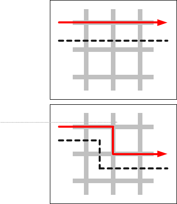
Major Traffic Flows

Another factor that should be considered when considering intersection groupings is

traffic-flow demand paths. With an arterial, this issue is moot, but with a grid

network, it can be crucial. With the grid pattern shown in the top chart in Figure 3,

the horizontal dashed line shows a likely group boundary. However, when a major

traffic-flow pattern does a dogleg, as shown in the bottom chart of Figure 3, then a

different group boundary may be appropriate. This characteristic will probably

manifest itself in the index, but when the signal engineer must make decisions

based on sparse data, then knowledge of traffic-flow patterns can be a useful

discriminator to identify group boundaries.

Figure 3. Grid Pattern.

Coordinatability Factor

There is one additional technique than can be employed by those that use the

computer program, Synchro. Synchro has an internal methodology to calculate a

“coordinatability factor.” This factor considers travel time, volume, distance, vehicle

platoons, vehicle queuing, and natural cycle lengths. The coordinatability factor is

similar to the “strength of attraction,” but also considers the natural cycle length

and vehicle queuing. The natural cycle length is defined as the cycle at which the

intersection would run in an isolated mode or the minimum delay cycle length. The

potential for vehicle queues exceeding the available storage is also considered in

determining the desirability of coordination.

Number of Timing Plans

The “rule of thumb” for the number of signal timing plans is that each group requires a

minimum of four plans: morning peak plan, average day plan, afternoon peak plan, and

evening plan. But each signal group is unique, and each group has unique demands. For

example, an arterial that provides access to a regional shopping center may experience

major demands on Saturday. Other examples abound of locations that require different

timing plans to meet demands by other major traffic generators, such as amusement parks,

recreational demands, and other non-work-related trips.

One analytical method that can be used to estimate the need for a special timing plan is to

plot the arterial traffic by direction and by time of day. The plot of the sum of both

directions provides an indication when cycle length changes may be required. Longer cycles

are typically required to service heavier volumes. The ratio of one direction to the total

traffic by time of day provides a good indication when offset changes may be required. The

number of plans required and the time during which they will be used is needed to schedule

the site surveys described in the next section. Analysis of the traffic demands at individual

intersections will indicate when split changes are required.

Cycle Length Issues

As noted above, having a common cycle length is fundamental to coordinated signal

operation. The cycle length must be evaluated from two different perspectives: individual

intersection and the group cycle length.

For the individual intersection, the recommended approach is to focus on the one or two

major intersections in the group—the intersections with the highest demand because these

are the ones that will set the minimum cycle length limits. When evaluating cycle lengths,

it is important to verify that the pedestrian timing is sufficient to allow pedestrians to cross

the street. When the pedestrian timing is known, say 7 seconds to Walk, 10 seconds for

pedestrian clearance, and 3 seconds for yellow change, and the vehicle phase is to be

allocated at least 25 percent of the cycle, then the minimum cycle length that can meet both

constraints is 20 seconds divided by 25 percent, or 80 seconds (assuming two critical

phases).

In general, the intersection in the group that requires the longest cycle length will set the

group cycle length. The cycle length and splits can be determined by using either Webster’s

equation or the Greenshields-Poisson Method. Both of these methods are explained below.

In general, for a given demand condition, there is a cycle length that will provide the

optimum two-way progression. This cycle length is a function of the speed of the traffic on

the links between intersections and the link distance between intersections. This cycle

length is called the “Resonant Cycle,” and is explained further below.

Webster’s Equation

One approach to determining cycle lengths for an isolated, pre-timed location is

based on Webster's equation for minimum delay cycle lengths. The equation is as

follows:

Cycle Length = (1.5 * L + 5) / (1.0 - Y

)

Where:

L = The lost time per cycle in seconds.

= Sum of the degree of saturation for all critical phases.

This method was developed by F. V. Webster of England’s Road Research

Laboratory in the 1960s. The research supporting this equation is based on

The critical phases are the ones that require the most green time. The flow ratio is calculated by

dividing the volume by the saturation flow rate for that movement.

measuring delay at a large number of intersections with different geometric designs

and cycle lengths. These observations yielded the equation that is used today. It is

important to recognize that this work assumed random arrivals and fixed-time

operation—two conditions that can rarely be met in the United States. Notice that

the equation becomes unstable at high levels of saturation and should not be used at

locations where demand approaches capacity. Nevertheless, this technique provides

a starting point when developing signal timings. To use this equation:

1. Estimate the lost time per cycle by multiplying the number of critical phases

per cycle (2, 3, or 4) by 5 seconds (estimated yellow change plus red clearance

time) to determine the “L” factor. L will have a value of 10, 15, or 20, and

the numerator will equate to 20, 27.5, or 35 seconds.

2. Estimate the degree of saturation for each critical phase by dividing the

demand by the saturation flow (normally 1,900 vehicles per hour per lane).

3. Sum the degree of saturation for each critical phase and subtract the sum

from 1.0. This is the denominator.

4. To obtain the cycle length, round the division to the next highest five

seconds.

Greenshields-Poisson Method

This approach to signal timing is statistically-based and makes several assumptions

about the behavior of traffic. It uses the Poisson distribution to describe the arrival

patterns of vehicles at an intersection. This distribution assumes that the vehicles

travel randomly. This assumption is frequently a problem in urban areas, but like

other methods, it can provide a good starting point to develop signal settings.

While the Poisson distribution is used to estimate the arrivals, the time required for

the approach discharge is based on work done by B. D. Greenshields in 1947.

Surprisingly, this work has held up well during the intervening 50 years. Like

Webster, Greenshields founded his work on many observations of traffic

performance. The results of these studies are summed in the equation:

Phase Time = 3.8 + 2.1 * n

Where:

Phase Time is the required duration to service the queue.

n is the number of vehicles in queue in the critical lane.

The basic procedure is iterative and uses the following steps:

1. Assume a cycle length. For two critical phases, we suggest 60 seconds; for

three critical phases, we suggest 75 seconds; and for four critical phases, we

suggest 100 seconds.

a. Calculate the number of cycles per hour by dividing 3,600 (seconds per hour)

by the assumed cycle length.

The critical lane or movement for each phase is the lane that requires the most green time.

2. For each critical phase, divide the demand volume by the number of lanes

and by the number of cycles per hour to determine the mean arrival rate per

lane.

3. Use the Poisson distribution (Table 1) to convert the mean arrival rate to the

maximum expected arrivals at the 95 percentile level.

4. Convert this maximum expected arrivals to time required using Greenshields

equation.

5. Add the time required for each critical phase plus the clearance and change

time required (nominally 5 seconds) for each critical phase. If the sum is

more than 5 seconds less than the assumed cycle, repeat the steps starting

with the new (shorter) cycle length. If the sum is greater than the assumed

cycle length by more than 5 seconds, repeat the steps but use the 90

or 85

percentile maximum expected arrivals. If the calculations using the 85

percentile arrivals indicate a cycle length greater than 80 seconds for two-

phase operation, 100 seconds for three critical phases and 120 seconds for

four critical phases, then the volumes may be too high to use this method.

Table 1. Poisson Distribution.

Mean Arrival Rate 85 Percentile 90 Percentile 95 Percentile

1 3 3 3

2 4 4 5

3 5 6 7

4 7 7 8

5 8 8 9

6 9 10 11

7 10 11 12

8 11 12 13

9 13 13 15

10 14 15 16

11 16 16 17

12 16 17 18

13 17 18 20

14 18 19 21

15 19 20 22

16 21 22 23

17 22 23 24

18 23 24 26

19 24 25 27

20 25 26 28

The Greenshields-Poisson Method is best suited to lower volume intersections.

When the critical lane volume exceeds 400 vph, then the basic assumption of

random arrivals (no vehicle interactions) is probably not valid. Even within this

range, care must be exercised. The method is designed to accommodate more

vehicles than is expected on average; but some percentage of the time, 5 to 15

percent, the demand will exceed the time allocated and not all arrivals will be

served. Care should be used to not apply this method at congested locations as the

process will suggest unrealistically long cycle lengths, which will result in high delay

and long queues.

Cycle Length

When the traffic demand is balanced in both directions on the arterial, and when

the distance between the intersections is approximately equal, then it is possible to

obtain good progression in both directions by adjusting the cycle length using the

following formulas:

(1) Cycle = 2 * Distance / Speed (1)

(2) Cycle = 4 * Distance / Speed (2)

(3) Cycle = 6 * Distance / Speed (3)

Where:

Cycle is the cycle length in seconds.

Distance is the link length in feet.

Speed is the average link speed in feet per second.

These equations define resonant cycle lengths for this signal group.

Notice that the

only real-time variable in the equations is traffic speed, which is actually used to

estimate link travel time. This implies that different cycle lengths would be

appropriate when there is a significant change in the link speed. It is typical for

link speeds to be slower during the peak periods. This implies that it may be

appropriate to use a longer cycle length during peak periods.

Once an appropriate cycle length is selected using one of the three formulas noted

above, the offsets can be identified as follows:

Formula (1) – The offset of an intersection at one end of the arterial is set to an

arbitrary value—many engineers use 0 seconds. The offset at the next intersection

is set to the sum of the value of the offset at the first intersection plus 50 percent of

the cycle. For example, if the offset of the first intersection is 0 and the cycle length

is 100 seconds, then the offset of the second intersection is 50 seconds. The offset of

the third intersection and all other odd-numbered intersections is the same as the

offset at the first intersection, 0 seconds in the example. The offset at the fourth

intersection and all other even-numbered intersections is the same as the offset at

the second intersection, 50 seconds in the example. This method of setting signal

timing is called a Single Alternate, and is the most desirable because it provides the

maximum bandwidth in both directions.

Formula (2) – The offset of two intersections at one end of the arterial are set to an

arbitrary value—0 seconds, for example. The offset at the next two intersections are

set to the sum of the value of the offset at the first intersection plus 50 percent of

“Resonant Cycles in Traffic Signal Control,” Shelby, S.G., Darcy Bullock, and Douglas Gettman,

TRB Meeting, January 2005.

the cycle. For example, if the offset of the first and second intersection is 0 and the

cycle length is 100 seconds, then the offset of the third and fourth intersections is 50

seconds. The offset of the fifth and sixth intersections is the same as the offset at

the first and second intersection, 0 seconds in the example. The offset at the

seventh and eighth intersection is the same as the offset at the third and fourth

intersections, 50 seconds in the example. The offsets at additional intersections are

in a similar manner. This method of setting signal timing is called a Double

Alternate, and is useful when the intersections are spaced more closely. It provides

bandwidths half that provided by the Single Alternate solution.

Formula (3) – The offsets at three intersections at one end of the arterial are set to

an arbitrary value—for example, 0 seconds. The offset at the next three

intersections are set to the sum of the value of the offset at the first intersection plus

50 percent of the cycle. For example, if the offset of the first, second, and third

intersection is 0 and the cycle length is 100 seconds, then the offset of the fourth,

fifth, and sixth intersections is 50 seconds. The offset of the seventh, eighth, and

ninth intersection is the same as the offset at the first, second, and third

intersection, 0 seconds in the example. The offsets at additional intersections are

set in a similar manner in groups of three. This method of setting signal timing is

called a Triple Alternate. This is appropriate for closely spaced intersections and

provides a bandwidth one-third that of the Single Alternate.

The important point to recognize when testing various Resonant Cycle lengths is

that the speed of traffic is set based on what the average driver considers

reasonable, not on an arbitrary speed that provides the maximum bandwidth. It is

a common error to put a timing plan in the field that looks great on paper, but does

not work in the field because the vehicles are traveling faster (or slower) than the

assumptions. Another related issue is that the average speed is not necessarily

consistent throughout the day. It may be lower during the peak periods or at night,

for example. Small errors in speed estimates can result in very poor signal timing

(large offset errors), especially on suburban arterials where the distances between

intersections are large. For example, estimating a speed of 30 mph when in fact the

true speed is 35 mph will result in an offset error of 13 seconds on a 4,000-foot link.

Offset Issues

The offset is the heart of coordination signal timing. It is the difference in time from a

reference point in the cycle at the upstream intersection to the same point in the cycle at

the downstream intersection. This reference point is usually taken to be the beginning of

the main street green. The simplest offset to consider is the one-way offset. When the light

turns green at the upstream intersection and the platoon travels down the link, it is

desirable for the downstream controller to change to green when the platoon approaches.

This offset is appropriate for one-way streets and for situations when heavy demand in one

direction justifies ignoring counter-flowing traffic.

Notice that this explanation deals with one link between intersections. Except at the ends

of an arterial, the intersections on an arterial have one intersection upstream and another

intersection downstream. It is important to recognize that changing the offset timing at

one intersection affects the relative offset on four links. This is illustrated in Figure 4.

Offset

Figure 4. Offset Change Impacts.

In this example, the offset of the middle intersection is adjusted downward (earlier). Notice

that this impacts the right-bound traffic flowing to the right intersection, as well as the two

links of left-bound traffic.

There is always a temptation to adjust the offset at one intersection to accommodate

demand in one direction on one link without taking into account the effects of this change

on the other three links. One way to manually analyze the offset impacts is to use the Kell

Method described below.

One-Way Offset

For the predominant one-way flow situation, the expedient approach requires only

an estimate of the median travel time between intersections. The offset, expressed

in seconds, is set at the intersections farthest upstream to an arbitrary value—many

engineers use 0 seconds. The offset at the nearest downstream intersection is

determined by adding the travel time to the offset of the adjacent upstream

intersection. The travel time is estimated by dividing distance between the

intersections by the average speed on the link. This process continues until the

offsets of all intersections in the group have been determined.

Notice that this method of determining offsets is independent of the splits at each

intersection and the cycle length.

As a further refinement, many traffic engineers will provide sufficient time for any

standing queue to discharge before the arriving platoon. To do this, estimate the

total number of vehicles in queue (vehicles that arrive during the red and do not

turn right). Divide this number by the number of lanes, and multiply the result by

2.5 seconds. Subtract this total from the offset that was determined by the link

travel time. Adjusting for the average standing queue is referred to as the “Smooth

Flow Offset.” As with the basic offset calculation method, when adjusting for the

standing queues, start at the upstream intersection and work downstream

calculating each offset based on the upstream offset by adding the travel time and

subtracting the queue discharge time to the upstream offset at each intersection.

Two-Way Offsets (Kell Method)

The Kell Method is a technique that can be used to manually construct a time-space

diagram that results in balanced offsets in both directions. This technique is named

after its developer; Mr. James H. Kell, who was an instructor at University of

California, Berkley. The process is straightforward and requires a minimum input

of information. An estimate of the percent green for the main street for each

intersection, the average speed on the arterial, and the distance between

intersections are the only information required to use the technique. The products

of the method are the cycle length for the arterial and the offset for each intersection

that provides equal bandwidth in each direction. The process is as follows:

1. Prepare a scale drawing laying out the intersections along the bottom of the

page.

2. Draw a vertical line at the first intersection on the left.

3. Draw several cycles on the vertical line using a closed rectangle to represent

the percent of time that the signal is not green.

4. Draw a horizontal working line through the middle of either a green or not-

green.

5. Draw a line that slopes upward and to the right at the beginning of green at

the left-most intersection. The sketch would look something like that shown

in Figure 5.

Figure 5. Kell Method (Beginning).

6. Plot the cycle of the next intersection such that either the green or the not-

green (whichever causes the beginning of green to come closest to the sloped

line) is centered on the Working Line, as shown in Figure 6.

Figure 6. Kell Method (Continued).

7. Continue plotting the cycle for the remaining intersections by centering

either the green or the red. A completed diagram is shown in Figure 7.

Figure 7. Kell Method (Completed Diagram).

Notice that this technique forces a symmetrical solution that provides two-way

progression with approximately equal bandwidths in each direction. The final

step in the process is to determine the cycle length. In general, traffic will move

on an arterial at a speed that the drivers consider reasonable for the prevailing

conditions. The engineer must estimate this speed and use it to determine the

cycle length. Notice that the diagram shows that a vehicle requires

approximately 1 ½ cycles to travel from intersection “A” to “D” in either

direction. If the prevailing speed on the arterial were 35 mph, then an

appropriate cycle length would be 75 seconds. This is determined by noting that

it requires 1 ½ cycles to travel 5,800 feet, which is equivalent to 3,867 feet per

cycle. The cycle length is determined by dividing the distance (3,867 feet) by the

speed, 51.33 feet per second (35 mph), and the cycle is 75 seconds.

Split Issues

The split is the amount of time allocated to each phase in a cycle at each intersection. The

toolbox offers two ways to calculate splits manually, the Greenshields-Poisson method

previously described and the Critical Movement method that is described below.

Critical Movement Method

This method uses techniques that were employed in the 1984 Highway Capacity

Manual as a “Planning Analysis” (Figure 8) to estimate intersection capacity. We

have adapted elements of this analysis to use to develop traffic signal timing

parameters. To use this method, intersection turning movements, the signal

phasing, and the cycle length for the intersection must be known. The designer

must determine the effective demand for each phase by applying various adjustment

factors to reduce the demand to passenger car equivalents per lane.

Figure 8. Critical Lane Analysis Example.

For the purposes of preparing traffic signal timing plans, a high level of precision is

not needed. Traffic demand can vary plus or minus 20 percent in just a few minutes

at a given location. Also a variation of 20 percent from day to day is not unusual.

Our objective, therefore, is to develop timing plans that are robust and that will

perform well through a wide range of demand conditions. The following steps are

suggested:

1. If the left turn movement is not protected, multiply the left turn demand by

1.6.

2. If the number of trucks is known, multiply the trucks by 1.5.

3. Divide the traffic demand on the four major and left-turn approaches by the

number of lanes for each movement.

4. Determine the critical movements for both the east-west street and the north-

south street. Determine the intersection critical movement by adding these

two together. If this sum is less than 1,500, then continue. If it is over 1,500,

then the intersection is probably over-saturated and the method may not be

applicable.

5. Determine the number of critical movements in each cycle. With no left-turn

protection, there would be two; with left turn protection on one street, there

would be three; and with left turn protection on both streets, there would be

four. Multiply the number of critical movements by five (the lost time), and

subtract this number from the cycle length. This result is an estimate of the

total available seconds of green per cycle that can be used for traffic

movements.

6. The final step is to multiply the total available green time by the ratio of the

critical lane volume for the movement to the total intersection critical lane

volume. For pre-timed operation, this is the phase green time in seconds.

For coordinated operation with actuated controllers, this phase time is used

to set the force-off for the phase. For all actuated phases, the calculated time

is the average green time for the phase. The phase maximum should be set

at 25- to 50-percent greater than this value.

IV. Local Controller Parameters

It is useful to identify traffic signal timing parameters as being in one of two categories:

local intersection timing parameters and coordinated operation timing parameters. The

phase minimum or yellow change times are examples of local intersection timing

parameters. The intersection cycle length and offset are examples of coordination timing

parameters. There are far more local intersection timing parameters than coordination

timing parameters. In fact, most systems define only three coordination timing

parameters: cycle length, offset, and split. The following section of this report describes

methods that can be used to set the local intersection timing parameters, while the next

section deals with the coordinated operation parameters.

The basic timing parameters are essentially the same for all actuated controllers. There

are subtle differences between different software implementations; for example, the NEMA

controllers define the force-off function as a “per ring” function, while other

implementations define the force-off function as a “per phase” function. This distinction has

little importance to the traffic engineer who is responsible for developing new traffic signal

plans. These differences, however, are very important when the results of a signal timing

optimization process are implemented in a particular controller. Many newer controllers

automatically calculate the force-off setting once the engineer defines the split.

Because most jurisdictions use NEMA TS-1 and TS-2 or Model 170 actuated controllers, the

primary emphasis has been placed on timing actuated controllers. It is important to

recognize, however, that many jurisdictions use pre-timed controllers. Most of the

principles noted in this section can be directly applied to pre-timed controllers.

For the current status on signal timing, the reader is directed to Signal Timing Practices

and Procedures: State of the Practice (Item IR-116) published by the Institute of

Transportation Engineers (ITE). This report documents the current state-of-the-practice in

traffic signal timing. It was prepared as part of a continuing program developed by FHWA

and ITE to place increased emphasis on the quality of U.S. traffic signal timing.

Actuated Controller Timing Principles

Some of the basic principles of timing the green interval in a traffic actuated controller unit

are as follows:

• Each phase must have a minimum green time so that a stopped vehicle that receives

a green signal has enough time to get started and partially cross the intersection

before the yellow signal appears. This time is sometimes called the initial portion of

the green interval.

• Each vehicle requires enough green time to travel from the detector to the

intersection. This is called passage time, vehicle extension, or gap. Gap refers to

the distance between vehicles as well as the time between vehicles. Each successive

vehicle actuation, therefore, increases the phase green time. With no opposing calls,

the controller rests. Extensions continue to be timed, but with no effect on the green

interval.

• There must be a maximum time that the green interval can be extended if opposing

cars are waiting; this is called the maximum green or extension limit.

• Once an actuation is received from an opposing phase, the maximum green timer

begins. The current phase will hold the green until the time between actuations is

greater than the preset unit extension or gap. When a gap is detected, the yellow

change interval will begin and the controller will transition to the next phase in

sequence with demand. This is called termination by gap or gap-out.

• An actuation from another phase received during any portion of the green interval

also starts the maximum green timing circuit. This is also called the extension limit.

Even if actuations are close enough in time to prevent gap termination, the

maximum limit will terminate the green interval when the preset maximum expires.

This is called termination by maximum green or max-out.

Basic Actuated Phase Settings

All actuated controllers support these five basic, phase-timing parameters: minimum

green, extension, maximum green, yellow and red.

Minimum Green (Initial)

The minimum green is the first timed portion of the green interval. The duration of

the minimum green is generally based on the number of vehicles that can be in

queue between the upstream phase detector and the stop line. In general, the phase

duration must be no shorter than some absolute minimum time, such as 5 to 10

seconds. If pedestrians may be crossing with this phase, their crossing time must

also be considered and included in the minimum phase length.

The term, minimum green, is called “minimum initial” on some controllers. There is

a subtle difference. The minimum green defines the duration of the green when

there are no extensions. When the controller uses a minimum initial, the minimum

green duration is equal to the sum of the minimum initial and one extension.

The minimum green time is the minimum assured green that will be displayed. It is

established to allow vehicles that are stopped between the detector on the approach

and the stop line to get started and move into the intersection. Therefore, timing of

this interval depends on the location of the detector and the number of vehicles that

can be stored between the detector and the stop line.

Consideration must also be given to pedestrian timing. When there are no

pedestrian provisions (indications or pushbuttons), the minimum assured green

must be equal to the minimum pedestrian timing (walk + pedestrian clearance).

One method that can be used to calculate the minimum green is:

Minimum Green = 5 + 2n

Where:

“n” is the number of vehicles that can be stored between the stop line

and the far detector in one lane. This is determined by dividing the

distance (in feet) between the stop line and the detector by 25, since 25

is the average vehicle length plus stopped-headway in feet.

When stop-line detection is used, the minimum green can be quite short, say 5 to 10

seconds. These very short minimums can be used on phases where there are no

pedestrian movements, and on phases where there are actuated pedestrian signals.

These extremely short minimums should never be used where there is the possibility

of pedestrians crossing with the green display.

Extension (Passage)

The extension (passage) parameter extends the green interval for each vehicle

actuation up to the maximum green. It begins timing when the vehicle actuation is

removed; that is, when the vehicle passes over the detector. This extension period is

subject to termination by the maximum extension timer or a force-off.

The actual passage time parameter (vehicle extension or gap time) is the time that

the phase will be extended for each actuation. This setting is the number of seconds

required for a vehicle moving at the approach speed to travel from the detector to

the stop line. The passage time serves two purposes: (1) it is the passage time from

the detector to the stop line, and (2) it is the allowable time gap between actuations

that will cause the green to remain on that approach. As long as vehicle detections

come at shorter intervals than the passage time (allowable gap), the green will be

retained on that phase until the maximum expires or it is forced-off.

If the passage interval is too short, quick stops may result as well as terminating the

green before the vehicular movement has been adequately served. If the passage

interval is set too long, excessive delays will result as well as safety problems due to

improperly timed last vehicle intervals.

Passage time is calculated as follows:

Passage Time = D / S

Where:

D is the distance from the stop line to the detector in feet.

S is the speed on the approach in feet per second.

Maximum Green

This time setting defines the maximum length of time that a phase can be green in

the presence of a conflicting call. If there is no conflicting call, it will be reset until

an opposing call occurs.

The maximum green timer is normally inhibited during coordinated operation when

the phase maximum time is determined by the phase force-offs. For most actuated

phases, the maximum green should be considered a safety constraint—something to

force the phase to end in the face of continuous demand. There is no accepted

practice to determine the optimum setting. Some engineers feel that all phases

should have similar limits like: 120 seconds for the primary through phases, 90

seconds for the secondary through phases, and 60 seconds for the left-turn phases.

Others set the phase maximums proportional to demand during a critical period.

For example, one could calculate the phase splits using the Critical Movement

method, then set the maximum green at 50-percent higher than the phase splits.

Yellow

The yellow interval follows the green interval at the end of each phase. The yellow

interval is also referred to as the “change” interval, and controls the duration of the

yellow display for that phase. The phase change interval timing advises drivers that

their phase has expired and they should: (1) come to a safe stop prior to the stop

line, or (2) proceed through the intersection if they are too near the intersection to

stop.

The following equation is generally used to determine the proper change interval:

Yellow Time = t + S / (2a +- 64.4 g)

Where:

t is the perception/reaction time of the driver in seconds (typically 1.0

second).

S is the speed on the approach in feet per second.

a is the deceleration rate in feet per second (typically taken as 10 feet

per second squared).

g = approach grade, percent of grade divided by 100 (add for up-grade

and subtract for downgrade).

Red

The red clearance interval (also known as the all-red interval) follows the yellow

interval of each phase. It must expire before the next phase in sequence can begin.

It is normally one to two seconds, but on slower speed approaches, it is not unusual

to use a very short duration of 0.0 to 0.5 seconds since the yellow time of 3.0 to 4.0

seconds provides sufficient time to meet both the change and the clearance

requirements.

Red Time = (W + L) / S

Where:

W is the Width of intersection in feet.

L is the length of vehicle in feet (typically taken as 20 feet).

S is the speed on the approach in feet per second.

Pedestrian Parameters

There are two pedestrian timing parameters: Walk and Flashing Don’t Walk (pedestrian

clearance). Where pedestrian movements regularly occur, pedestrians should be provided

with sufficient time to cross the roadway (MUTCD section 4D.03). In other words, unless

the pedestrian movement is actuated, the time required for pedestrians to safely cross the

road (the sum of the Walk and Don’t Walk times) will dictate the minimum green time for

that phase. When pedestrian pushbutton (actuation) is provided, then the normal vehicle

minimums would be used in the absence of a pedestrian actuation. Notice that it is possible

to have a signal design that uses pedestrian pushbutton detection without using pedestrian

Walk and Don’t Walk displays.

Walk

The Walk parameter controls the length of time that the walk signal is displayed.

Under normal conditions, the walk interval is 4 to 7 seconds. This allows

pedestrians to have adequate opportunity to leave the curb before the clearance

interval is shown. Under special circumstances, such as at a school crossing with

numerous pedestrians, walk times may exceed 7 seconds. Research indicated that

pedestrian queues of 24 or more people can be accommodated in 7 seconds.

Flashing Don’t Walk

The pedestrian clearance parameter controls the duration that the Flashing Don’t

Walk is displayed. This is the time required for a pedestrian crossing in the

crosswalk to leave the curb and travel out of the traveled way (MUTCD section

4E.02) before opposing vehicles receive a green indication.

The Flashing Don’t Walk (pedestrian clearance) is calculated as follows:

Flashing Don’t Walk = W / S

Where:

W is the walking (crossing) distance in feet from curb to curb.

is the average walking speed in feet per second (typically 3.5 to 4

feet per second).

Volume-Density Phase Settings

In the 1950s, the Automatic Signal Company introduced two new and complex traffic signal

controllers, the Model 1022 and the Model 1033. These controllers had far more timing

circuits than any controllers used before or since. Although all of the timing parameters

were well-founded in theory; in practice, many did not actually improve the performance of

the intersection. There were several reasons for this experience: it was not possible to

determine which of the many timers actually caused a particular phase to terminate; the

analog timing circuit technology available at the time was subject to variations based on

temperature and humidity; and like today, few engineers had the time necessary to fine-

tune the operation. Of the many features of these innovative controllers, two features

(variable initial and gap reduction) have evolved and are typically available with today’s

controllers. These two features are explained below.

Variable Initial

To successfully employ the volume density features of a controller, it is necessary to

have phase detection farther upstream than that which is normal. This enables the

controller to sample traffic on the approach with a minimum impact from a standing

queue. Detection 300 to 400 feet upstream from the stop line is typical with volume

density operation. With detection this far back, the minimum green would be quite

long—35 seconds with the detector back 400 feet. Since a minimum green this long

would result in very sluggish operation when the demand is light, two other timing

circuits are used to mitigate these impacts: Added Initial and Maximum Initial.

Added Initial – This interval times concurrently with the minimum green interval.

The value is the amount of time that is added when each vehicle actuation is

received during the initial period. The actual minimum green time used by the

controller is the greater of the minimum green or the added initial sum. The added

initial cannot exceed the maximum initial. The added initial allows the duration of

the minimum to vary between the actual minimum and the time required to

discharge the maximum queue that can be stored between the stop line and the

detector.

Maximum Initial – This is the maximum period of time for which the added initial

can extend the initial green period. The maximum initial cannot be less than the

minimum green.

Gap Reduction

Gap reduction is the other legacy concept that is used on the modern controller.

This parameter is used to allow the “gap seeking” logic of the actuated controller to

identify a smaller gap in traffic to justify terminating the phase earlier than that

which is implied by the passage time. Gap reduction is a means of reducing the

passage time or gap on the basis of the time that opposing vehicles have waited. In

effect, it benefits the waiting vehicles by reducing the time allowed between vehicles

arriving on the green phase before that phase is terminated. There are three timing

parameters associated with the gap reduction feature: Time-Before-Reduction, Time-

to-Reduce, and Minimum Gap.

Time-Before-Reduction – This period begins when the phase is green and there is

a serviceable call on a conflicting phase. When this period is completed, the linear

reduction of the passage time begins.

Time-To-Reduce – This period begins when the time-before-reduction ends, and

controls the linear rate of reduction until the gap is reduced to the minimum gap.

Minimum Gap – Like the passage time, this parameter extends the green interval

by the minimum gap time for each vehicle actuation up to the maximum green. It

begins timing when the vehicle actuation is removed. This extension period is

subject to termination by the maximum green or a force off.

Controller Timing Parameters Summary

There are 12 controller timing parameters that are commonly used:

1. WALK Establishes the length of the Walk interval.

2. PED CLEARANCE Establishes the length of flashing Don’t Walk interval.

3. MINIMUM GREEN Establishes the length of initial state of green interval.

4. PASSAGE TIME Establishes the increment of right-of-way (green) time

extension for each vehicle actuation during the green

interval.

5. MAXIMUM GREEN Establishes the maximum limit to which the green

interval can be extended on a phase in the presence of a

serviceable demand on a conflicting phase.

6. ADDED INITIAL Density feature. Establishes number of seconds by

which each vehicle (actuation) increases the initial state

of green during non-green time on the phase.

7. MAXIMUM INITIAL Density feature. Establishes the maximum limit to

which the initial interval can be extended on a phase.

8. TIME B4 REDUCTION Density feature. Establishes a preset time before the

allowed gap (passage time) begins to reduce.

9. TIME TO REDUCE Density feature. Establishes time in which the allowed

gap is reduced from passage time to minimum gap, after

the time before reduction has expired.

10. MINIMUM GAP Density feature. Establishes minimum value to which

allowed gap between actuations on phase with green can

be reduced upon expiration of time to reduce.

11. YELLOW CHANGE Establishes the length of yellow interval following the

green interval.

12. RED CLEARANCE Establishes the length of red clearance interval following

the yellow interval.

V. Coordination Timing Issues

There are three parameters that determine how a controller functions in a coordination

mode: cycle length, offset, and split. While all three parameters are important to the

efficient operation of a signalized arterial or network, it might be argued that the cycle

length is the most important of these parameters because it determines the periodicity of

the system.

Resonant Cycle

In the discussion of the cycle length, we introduce the concept of the resonant cycle length

That is, for regular linear and grid networks, there are one, two, and sometimes three cycle

lengths that provide much better operation than other cycles. In other words, the concept

of a resonant cycle is a cycle length that accommodates good two-way progression. The

resonance (and non-resonance) of a cycle time stems from the principle that intersection

spacing precludes good progression at certain cycle lengths, and conversely, some cycle

lengths necessarily preclude progression on an arterial due to their incompatibility to the

network geometry. The second essential element of a resonant cycle is that it continues to

provide good two-way arterial progression over a range of volumes.

Resonant cycles naturally arise on arterials as a function of what cycle provides good two-

way progression for given intersection spacing, vehicle speeds, volume levels, saturation

flow rates, and phase sequencing. Time-space diagrams can be used to provide a

convenient means of conveying the traffic flow mechanics that give rise to the resonant

cycle. The results of the experiments, taken as a whole, suggest that well-chosen cycle

lengths scheduled by time-of-day or selected from a table dynamically could yield better

progression, delay, and travel time performance than an on-line incremental adjustment

strategy based on maintaining a constant, target degree of saturation for the single most

congested intersection—a typical adaptive control strategy.

Optimizing an arterial signal-timing plan (cycle, splits, and offsets) for a singular set of

input volumes can be handled in a straightforward manner by using signal-timing

optimization software such as Transyt-7F or Synchro. However, a much more challenging

task is compiling a set of time-of-day (TOD) signal-timing plans and a TOD schedule for

each day of the week to accommodate all hourly and daily fluctuations in traffic conditions

typically experienced during the week.

There are currently no commercially available off-the-shelf tools to address this problem,

and even the literature offers very little in terms of structured guidance to accomplish this

task. The decisions to be made include the following:

• Select a workable number of plans. For example, 15 signal-timing plans usually are

not practical. A typical day might minimally consist of four plans: the AM peak, PM

peak, off-peak day, and off-peak night. Also, for areas in the vicinity of major

shopping facilities, one might consider a special plan to accommodate shopping

traffic demand.

“Resonant Cycles in Traffic Signal Control,” Shelby, S.G., Darcy Bullock, and Dougles Gettman,

TRB Meeting, January 2005.

• Construct a schedule. Each hour of the week must be covered by a signal-timing

plan. For example, the schedule determines when the AM peak plan starts and ends,

subsequently switching to the off-peak plan.

• Determine the input volumes to generate each plan. Over the hours that each

signal-timing plan will be in operation, traffic conditions may fluctuate significantly.

However, signal-timing optimization software only accepts a single set of input

volumes to generate a corresponding plan. For example, a user might use the peak-

hour flows observed over the whole time frame a plan will be in effect.

The decisions are all interrelated. For example, the number of workable plans may depend

on the number of “distinct” traffic conditions that can be discerned. The construction of the

schedule will depend on the number of timing plans that are appropriate through a given

day. The input volumes will depend on what time of day a plan is in effect. Until very

recent publications, engineering judgment was the only guide to making these decisions.

A paper published in 2002 suggests that a statistical clustering algorithm, based on

volumes approach to the arterial’s critical intersection, be used to determine “break-points”

(or switch points) between TOD plans in the daily schedule.

A subsequent paper, published in 2004, suggested flaws with using volume clusters and

recommended that 90th percentile volumes (of a set of several TOD observations) of the

critical intersection be used instead to optimize its cycle length based on a uniform delay

equation.

These plans would then be evaluated over several TOD intervals (using a

genetic algorithm) to optimize the TOD schedule of the critical intersection.

Intersection Categories

In the signal network to be retimed, all intersections can be divided into two categories:

primary intersections and secondary intersections. The primary intersections have the

highest demand-to-capacity ratio and will, therefore, require the longest cycles. These

intersections are usually well-known to the traffic engineer. They are the intersection of

two arterials, the intersections with the worst accident experience, the intersections that

service the major shopping centers, and the intersections that generate the most

complaints. The secondary intersections generally serve the adjacent residential areas and

local commercial areas. They are usually characterized by heavy demand on the two major

approaches and much less demand on the cross-street approaches.

The purpose of assigning intersections to one of these two categories is to reduce the

locations where traffic counts are required. The primary intersections require turning

movement traffic counts—there is simply no other way to measure demand. However, the

secondary intersections usually have side street demand that can be met with phase

minimum green times. The strategy, therefore, is to concentrate the counting resources at

Smith, B. L., W. T. Scherer, T. A. Hauser, and B. Park, “Data-Driven Methodology for Signal Timing Plan

Development: A Computational Approach,” Computer-Aided Civil and Infrastructure Engineering, Vol. 17, 2002,

pp. 287-395.

Park, B., P. Santra, I. Yun, and D. Lee, “Optimization of Time-of-Day Breakpoints for Better Traffic Signal

Control,” TRB 83rd Annual Meeting Compendium of Papers. CD-ROM. Transportation Research Board, National

Research Council, Washington, D.C., 2004.

the locations where there is no substitute, and to use minimum green times for the minor

phases at secondary intersections.

Number of Timing Plans

A unique timing plan is required whenever a cycle length, offset, or split is different from

the previous setting. When a new timing plan is selected, the controller must “transition”

to the new plan. During this transition period, systematic operation in the network is

interrupted while each controller adjusts to the new parameters. Because of this

disruption, transitions are minimized and one must be assured that the benefits of the new

plan overcome the disbenefits of the transition period.

One way to determine how many timing plans are needed is to assume that a new plan is

needed whenever there is a significant change in the traffic demand. This may be assessed

by evaluating the changes in demand by hour and by direction. For the network, array the

northbound, southbound, eastbound, and westbound in a table where the directional flows

are in columns and the rows represent the hourly data. Have a column of the table

represent the sum of the four directional flows. Examine this column to identify the time

during which there is a significant change in the total demand; this is an indication that

different cycle length (new timing plan) may be warranted.

Assuming that the major flows are on the north-south street, calculate the basic split by

dividing the greater of the northbound or southbound by the total intersection demand for

the period. When this ratio changes is a good indication of the need for a new plan to

accommodate a new offset. Periods when a new plan may be warranted are identified by

the changes in either the total demand or the split demand.

Using the Tool Box

We have placed a significant emphasis on discussing resonant cycle lengths because plan

changes involving different cycle lengths are very disruptive during the transition period.

In contrast, timing plan changes that involve different offsets with the same cycle length

are relatively benign, and plan changes that only involve split differences are generally

unnoticed. It is important, therefore, to identify the resonant cycle and use this cycle for as

many plans as possible.

When a computer model is not available, we suggest that the following procedure be

followed:

1. Cycle – For each primary intersection, calculate the cycle length required using

Webster’s equation as defined in Section 4.1. For each signal group, determine the

resonant cycle length using the equations provided in Section 4.2. Select the longest

cycle for the timing plan.

2. Split – For each primary intersection, determine the intersection splits using the

Critical Movement method explained in Section 4.5 and the selected cycle. For each

secondary intersection, determine the time required for each minor movement using

the Greenshields-Poisson method and the cycle explained in Section 4.6. Check both

primary and secondary intersections for pedestrian timing requirements and adjust

as necessary.

The purpose of obtaining count data is to use it as input to a timing model. The

timing model then generates the appropriate signal settings. There is an alternative

way, which is to estimate the settings directly. This is being performed when

estimating the minimum phase time for the cross-street movements at a secondary

intersection. The turning movement data at the primary intersection might show

that the cycle length for the group should be 100 seconds. If we allow a phase

minimum of 10 seconds and assume 5 seconds for the change and clearance

intervals, then we can determine that the side street split should be 15 percent. To

work the numbers another way, there will be thirty-six 100-second cycles per hour.

Ten seconds is sufficient time to discharge three to four vehicles per cycle. In other

words, this strategy will provide enough capacity to discharge approximately 125

vehicles per lane in an hour. As long as the demand is less than the 125 vehicles per

lane, this approach will work fine.

This example describes one way to estimate secondary intersection split, given the

cycle length. For system timing, we must also have a means of estimating the third

parameter, the offset. We can do this for two conditions: when the demand in one

direction is predominant and when the demand is relatively balanced.

3. Offset – Determine the offsets using the Kell method as outlined in Section 4.4.

When using the Kell method (or any maximum bandwidth method), the practitioner

has several options. The most obvious, and most frequently used, is to consider an

arterial as single entity. This will generally result in balanced bandwidths in both

directions.

During periods of directional flow, however, it may be useful to consider a minor

variation. Within any arterial group, the signals can be clustered in subgroups. The

intent is to cluster signals that have similar link lengths into subgroups. The Kell

method is then applied to each cluster, which by virtue of the similar link lengths,

will have good progression in each direction. The offsets within the subgroups are

those generated by the Kell method. The offset between clusters is set using the

one-way method defined in Section 4.3 to favor the peak directional movement. This

technique assures good progression in the peak direction while providing good

progression within the clusters in the counter-flow direction.

During periods of heavy directional flow, it may be necessary to ignore the contra-

flow traffic to accommodate the peak directional demand. In this instance, all of the

offsets are developed using the one-way method as described in Section 4.3.

VI. Signal Timing Examples

One way to illustrate how the tools and techniques presented in this document can be used

to develop good signal timing plans on a shoestring (low budget) is to provide an example.

Three different examples are discussed illustrating different measures that could be used

depending on the available resources.

Moderate Signal Timing Budget

In this example, an agency retained a consultant to prepare signal timing plans for a

suburban arterial three years ago when the arterial was widened and new controllers were

installed. The new timing plans worked well in the beginning, but as development

increased in the corridor, some obvious problems are beginning to emerge. Most of the

problems can be related to the opening of the new shopping center with major signalized

entrances at two of the 10 signals in the corridor. Although a consultant prepared the

existing signal timing plans, the agency required the consultant to develop the timing plans

using the same program that the agency uses, and required the consultant to deliver all of

the data input files for the program.

1 – Identify the System Intersections

In the example, this is obviously the 10 intersections described in the arterial.

2 – Collect and Organize Existing Data

This is a critical step in minimizing the cost of developing new plans. In the

example, one can assume that there are turning movement counts available for all

10 intersections—the only problem is that they are three years old and there have

been changes in the traffic demand in the corridor. Nevertheless, it is likely that

some of the existing turning movement data can be updated and used in developing

the new plans. However, new turning movement counts probably will be required

for the two intersections that are the entrances to the shopping center.

Another type of data that will prove to be very useful is a 24-hour directional count

on the arterial. The directional count can be used to estimate any overall change in

the traffic demand during the last three years. Factors developed using these data

can be used to adjust the three-year-old turning movement counts to reflect the

current demand.

The agency is fortunate in that other data that would normally be collected (e.g.,

distance between intersections, intersection geometry, signal phasing, and the like)

is already available and coded in the optimization program input files. For the most

part, the agency only has to update the traffic demand information and rerun the

program to obtain updated signal timing plans.

3 – Conduct Site Survey

Although many engineers are tempted to skip this step, experience has shown that a

visit to the site during the hours for which the timing plans are being developed can

be very beneficial.

Specific things to look for are unusual demand conditions. In the example, the

timing at the two intersections affected by the shopping center needs to be

updated—one might assume that the signal settings at the other eight intersections

may be pretty good. This can be confirmed by a quick trip to the location during the

peak periods. This field visit frequently exposes additional issues that can be

readily addressed with new timing plans.

4 – Obtain Turning Movement Data

This is the key step in minimizing the cost of developing signal timing plans. In the

example, assuming that the 24-hour data can be used to update the old turning

movement counts and that the site visit did not uncover a latent demand condition,

new counts would be needed only at the two intersections that are heavily impacted

by the shopping center. The 24-hour directional count data is used to reaffirm that

the arterial should continue to operate with four timing plans.

To obtain the turning movement data, the agency will conduct short counts during

the AM peak, PM peak, afternoon, and evening periods at the two locations. The

times when the short counts are scheduled are determined from the 24-hour

directional data. Factors developed from the 24-hour directional data are used to

update the existing turning movement counts at the remaining eight intersections.

5 – Calculate Local Timing Parameters

Because there is no significant change proposed to the operation of the individual

controller, there is no need to change any of the local timing parameters.

6 – Identify Signal Groupings

Because there is no need to change the structure of the system, there are no changes

required in the grouping of the signals.

7 – Calculate Coordination Parameters

Once the turning movement data are available, it is a simple matter to update the

input files and rerun the optimization program.

8 – Install and Evaluate New Plans

The physical installation of the new timing plan parameters is usually

straightforward, but a task that is done manually offers the potential for significant

errors. A major concern in the installation phase is verification that the optimized

parameters are, in fact, the parameters that are installed.

The second issue in this step is evaluation of how effective the new settings are. For

agencies that have some resources that can be applied to signal timing issues,

evaluation is an area that provides increasing benefits over time. To evaluate the

timing plans developed in this scenario, two separate types of studies are

recommended: travel time and stopped-time delay. The travel time studies of a

route up and down the arterial will provide a quantifiable measure of the traffic

performance in the corridor. To compliment this information, delay studies at

selected intersections will provide insight to the operation of specific intersections.

In the example, consider making delay studies at the two intersections where

entirely new plans were installed. In addition, it is appropriate to make delay

studies at the critical intersection in the group. The critical intersection is generally

the most congested; it is the intersection that drives the cycle length for the group.

The combination of travel time studies and delay studies will provide an excellent

baseline condition against which future changes in signal timing can be compared.

Modest Signal Timing Budget

The second example uses a similar geometric situation with an entirely different system

history. In this case, there is a 10-intersection arterial; but until now, all intersections have

operated as full-actuated, isolated signals. The agency has just hired an electrical

contractor to install new controllers, interconnect cable, and an on-street master. This is

the classical installation of a “closed loop” system. To save scarce funding, the agency plans

to develop the timing plans themselves and has limited resources for this effort.

1 – Identify the System Intersections

In this second example, it is obvious that the 10 intersections will constitute the

signal system.

2 – Collect and Organize Existing Data

The use of existing data is even more critical in minimizing the cost of developing

new plans. In this example, one can assume that there are turning movement

counts available for all 10 intersections, but the turning movement counts were

made during different years. Some of the existing counts are more than 10 years

old. While there have been changes in the traffic demand in the corridor over the

last 10 years, most of the development has taken place on the East side. It is likely

that some of the existing turning movement data at intersections on the West side

can be updated and used for developing the new plans. However, new turning

movement data will likely be required for the five intersections on the East side.

As with the first example, the 24-hour directional count on the arterial will prove to

be very useful. If a recent directional count is not available, one must be made as a

first step. Hopefully, there are older 24-hour counts that are available and can be

used to develop factors to adjust the existing turning movement counts to reflect the

current demand.

Although the available funds are modest, the agency owns a signal timing

optimization program and plans to use it. This decision may cost a little more in the

short run, but it will allow the agency to easily revise the signal timing plans in the

future when the input file is updated with new turning movement counts. In the

meantime, it is necessary to collect all of the descriptive required by the program.

This descriptive data includes the following:

• A condition diagram of each intersection showing the number of lanes and

width of each lane on all approaches. The condition diagram must have a

North arrow and show the street names.

• A phasing diagram for intersections with existing controllers. It is important

for the phasing diagram to include the NEMA phase number for each phase

movement. The phasing diagram must also show all overlaps (if any).

• Distance between intersections and the free-flow travel speed for the

conditions under which the timing plan will operate. This information should

be depicted on a map of the area showing the roads and signalized

intersections. It is not necessary for the map to be drawn to scale, but it is

important for each link on the map to be long enough to be able to show

various data such as link length, speeds, and volume.

With this information in hand, particularly the 24-hour directional count, the

engineer can begin making some difficult decisions concerning turning movement

data. A first step is to identify each intersection as either primary or secondary. As

previously noted, the primary intersections are the ones that are the most congested

and that drive the cycle length requirements. Another initial step is to determine

how many timing plans are required for the facility. Using the methodology that

compares total intersection and directional volume hour by hour is a good indication

of when new timing plans are needed.

The engineer has three options to obtain the turning movement data that is

necessary to run the optimization program: update the existing counts, make new

counts using short-count techniques, or estimate the turning movements using a

program like Dowling Associates’ TurnsW. With the provided scenario, one would

tend to update the intersections on the West side (lowest growth) and make new

short counts at the intersections on the East side. The estimated counts could be

used at secondary intersections on the West side if data collection costs were a major

limitation.

3 – Conduct Site Survey

To save time and cost, many engineers are tempted to skip this step. This would be

a mistake. Experience has shown that a visit to the site during the hours for which

the timing plans are being developed will be beneficial.

4 – Obtain Turning Movement Data

This is typically the most costly step in the signal timing process. After making the

best possible use of the existing data as previously described, this step provides for

the field data collection of turning movement counts.

5 – Calculate Local Timing Parameters

Because the existing controllers are operating in the full actuated mode, the local

timing parameters probably do not require any change.

6 – Identify Signal Groupings

Because there is no need to change the structure of the system, there are no changes

required in the grouping of the signals.

7 – Calculate Coordination Parameters

Once the turning movement data are available, it is possible to run the optimization

program.

8 – Install and Evaluate New Plans

The physical installation of the new timing plan parameters is usually

straightforward, but any task that is done manually offers the potential for

significant errors. A major concern in the installation phase is verification that the

optimized parameters are, in fact, the parameters that are installed.

The second issue in this step is evaluation of how effective the new settings are. For

agencies that have few resources, the evaluation frequently must be subjective.

Nevertheless, this element is a very important part of the signal timing process.

Rather than conducting formal travel time studies, the engineer may simply drive

the arterial several times looking for discontinuities in the traffic flow or congestion

where none was expected. These informal evaluations must be conducted during the

periods for which the timing plans were developed. The engineer should pay

particular attention to any instances of cycle failure (approach demand is not met

during a green phase) as an indication of a serious deficiency.

Minimum Signal Timing Budget

The third example involves developing signal timing with the absolute minimum of

resources. This example is similar to the previous example, except there are only five

intersections on the arterial and all are currently operating as isolated, actuated

controllers. However, the controllers have time-based coordination capability, and the

engineer wants to use this function.

In the previous examples, the cost of preparing the plans was minimized by reducing the

cost of the data collection effort necessary to run the optimization software, specifically, the

turning movement counts. With this absolutely minimalist approach, a different process is

used. Instead of estimating the input data, the process involves estimating the parameters

(cycle length, split, and offset) themselves using time-space geometry and estimates based

on engineering judgment.

1 – Identify the System Intersections

In the example, the system consists of the five intersections.

2 – Collect and Organize Existing Data

As with the previous examples, the practitioner must make maximum use of

existing data, especially existing timing data and system layout information.

3 – Conduct Site Survey

This step is absolutely vital with the minimalist approach. The practitioner must

carefully observe each of the five intersections for several cycles during the period

for which the timing plan is being developed. In this survey, the practitioner must

estimate the average speed of the traffic between intersections on the artery, and if

not available in the existing data, the practitioner must measure the distance

between intersections.

As with the previous examples, specific issues to look for are unusual demand

conditions, pedestrian demands, and any congested movements. The primary

output of this effort is the identification of the primary intersection in the group.

4 – Obtain Turning Movement Data

With the minimalist approach, the practitioner must obtain current turning

movement information for the primary intersection usually by using short-count

techniques as with the previous examples. In addition, the practitioner must obtain

24-hour directional counts on each of the four major approaches to the primary

intersection.

At secondary intersections, the practitioner must observe the operation of the

intersection for several cycles and record the average phase time for each phase

during the cycle.

5 – Calculate Local Timing Parameters

Unless a problem is identified during the site survey, there is usually no need to

change any of the local timing parameters.

6 – Identify Signal Groupings

Because there is no need to change the structure of the system, there are no changes

required in the grouping of the signals.

7 – Calculate Coordination Parameters

In the previous two examples, this step involved running an optimization program.

With the minimalist approach, this step involves estimating the coordination

parameters directly.

Cycle Length – The cycle length must be selected for the group based on meeting

three criteria: optimum cycle length, resonant cycle length, and pedestrian

constraints.

Using the turning movement information at the primary intersection, calculate the

optimum cycle length using Webster’s equation:

Cycle Length = (1.5 * L + 5) / (1.0 - Y

Using the intersection layout and phasing, determine the minimum pedestrian cycle

length:

Ped Minimum Cycle = LT + 14 + W

/ S

P +

/ S

Where:

LT = Time required for the left turn movements.

14 = (2 * 7) Time that the “Walk” is displayed to cross each street.

/ S

= Width of the main street divided by the pedestrian speed.

/ S

= Width of the cross street divided by the pedestrian speed.

Y = Yellow and All Red time for critical phases.

Using the average distance between the five intersections, calculate the potential

resonant cycles using the following equations:

Cycle = 2 * Distance / Speed

Cycle = 4 * Distance / Speed

Cycle = 6 * Distance / Speed

Cycle = 8 * Distance / Speed.

Select the shortest resonant cycle that is longer than the optimum cycle and the

pedestrian minimum cycle. If none of the resonant cycles are longer than the

optimum cycle, select the longest resonant cycle.

Offset – The offset is calculated using the Kell method.

Split – The split is calculated for the primary intersection using the Critical

Movement method. Once the splits are calculated based on demand, they must be

checked to verify that the pedestrian requirements are met. For example, assume

that the calculated splits required 15 seconds for phases 4 and 8. If the minimum

pedestrian time were 19 (7 + 48/4) seconds, then the intersection split would have to

be increased to 19 seconds to accommodate the pedestrian movement.

At intersections other than the primary intersection, the split is based on the

average phase time observations. These averages are converted to a percent of the

cycle, and new splits are calculated by multiplying these percent splits by the new

cycle length. The final split is based on the pedestrian requirement or the average

phase time, whichever is longer.

8 – Install and Evaluate New Plans

As with the other methods, the physical installation of the new timing plan

parameters is usually straightforward, but any task that is done manually offers the

potential for significant errors. A major concern in the installation phase is to verify

that the optimized parameters are, in fact, the parameters that are installed.

This minimalist approach takes many short cuts compared to the steps that would

be followed in a traditional signal timing effort. It is very important for the

practitioners to carefully verify these plans in the field. In fact, in spite of the

objective of minimizing costs, more time and effort should be planned for this task

under this approach than either of the two other approaches that use optimization

software. The new plans should be tested during a period of low traffic demand

conditions before they are used in the period for which they are designed. For

example, a plan for the AM rush hour might be tested in the late morning or early

evening when the demand is usually lighter. This test period should allow the

practitioner to identify any serious discrepancies without having a large negative

impact on traffic operations.

U.S. Department of Transportation

Federal Highway Administration

Office of Operations

400 7

Street S.W. (HOP)

Washington, DC 20590

Publication No.

FHWA-HOP-07-006