The Benefits of the Home Mortgage Interest Deduction

This PDF is a selection from a published volume from

the National Bureau of Economic Research

Volume Title: Tax Policy and the Economy, Volume

Volume Author/Editor: James M. Poterba, editor

Volume Publisher: MIT Press

Volume ISBN: 0-262-16220-2

Volume URL: http://www.nber.org/books/pote03-1

Conference Date: October 8, 2002

Publication Date: January 2003

Title: The Benefits of the Home Mortgage Interest

Deduction

Author: Edward L. Glaeser, Jesse M. Shapiro

URL: http://www.nber.org/chapters/c11534

THE BENEFITS

OF THE

HOME MORTGAGE

INTEREST DEDUCTION

Edward

Glaeser

Harvard University

and

NBER

Jesse

Shapiro

Harvard University

EXECUTIVE SUMMARY

The home mortgage interest deduction creates incentives

to buy

housing

and to

become

homeowner,

and the

case

for the

deduction rests

on social benefits from housing consumption

and

homeownership. There

is little evidence suggesting large externalities from

the

level

housing

consumption,

but

there appear

to be

externalities from homeownership.

Externalities from living around homeowners

are far too

small

justify

the deduction. Externalities from home ownership

are

larger,

but the

home mortgage interest deduction

is a

particularly poor instrument

for

encouraging homeownership because

it is

targeted

at the

wealthy,

who

are almost always homeowners.

The

irrelevance

of the

deduction

is sup-

ported

by the

time series, which shows that

the

ownership subsidy moves

with inflation

and has

changed significantly between

1965 and

today,

but

the homeownership rate

has

been essentially constant.

INTRODUCTION

The American subsidy

homeownership

among

the

most prominent

features

of our tax

code.

In 1999,

$773 billion

was

deducted

by 40

million

38 Glaeser

Shapiro

homeowners using

the

home mortgage interest deduction. After state

taxes,

it is the

most common deduction,

and it

stands

as one of the

most striking

and one of the

most debated features

of the U.S. tax

code.

its

detractors,

the

home mortgage interest deduction

is a

boondoggle

that robs

the U.S.

Treasury

and

subsidizes America's wealthiest home-

owners,

the

construction industry,

and

quite possibly politically active

banks

and

entities like Fannie

Mae and

Freddie

Mac. To

these critics,

the

deduction stands

glaring evidence

for

Director's Law—redistribution

ultimately goes

to the

median voter.

The

critics

of the

deduction argue

that

distorts behavior

and

induces Americans

spend

too

much

housing. Some analysts, such

Voith (1999), even blame

the

plight

the inner cities

on the

housing subsidy.

its

supporters,

the

home mortgage interest deduction

is a

corner-

stone

American society. Homeownership gives people

stake

soci-

ety

and

induces them

care about their neighborhoods

and

towns.

subsidizing property ownership,

the

deduction induces people

invest

and then

have

stake

in our

democracy. Ownership makes people vote

for long-run investments instead

short-run transfers. Home ownership,

and perhaps housing consumption

itself,

seems

to be

good

for the out-

comes

children.

The

deduction

may

favor

the

rich,

but

after

all,

much

the tax

code

progressive

and the

home mortgage interest deduction

levels

the

playing field

little.

We believe that there

truth

both views.

The

home mortgage interest

deduction, like almost

all

deductions, disproportionately favors

the

wealthy.

2001, more than

percent

taxes saved

deductions were

saved

by the

richest decile

America. Furthermore,

rich body

of eco-

nomic research shows

how the

deduction increases,

and

possibly distorts,

housing consumption.

However, there appear

to be

externalities both from homeownership

and from housing consumption

itself.

Causal inference

tricky,

but

homeownership

strongly correlated with political activism

and

social

connection. Homeownership appears

increase home maintenance

and

gardening. Most tellingly, people seem

to be

willing

to pay

live

around homeowners. Controlling

for

metropolitan area

and for the ob-

servable human capital

neighbors,

find that

a 10

percent increase

the

local homeownership rate increases local housing prices

by 1.5 per-

cent. While omitted unobservable variables might explain this correlation,

the overall body

research seems

confirm positive externalities from

homeownership.

The evidence suggests externalities that might

worth subsidizing,

but

the

home mortgage interest deduction does

not

appear

to be an

effec-

The Benefits of the Home Mortgage Interest Deduction 39

FIGURE 1. Homeownership and Inflation, 1965-2000*

—^-e—

First quarter homeownership *-• Subsidy

100

200

\ k

t -i Mi

'i I 1 e^o "

150

i • MM

£ : f s f \ MOO

« • | / ;

e • / ". " M A-&-^ \ r 50

1965

1970 1975 1980 1985 1990 1995

2000

Year

* Subsidy series shows the effect of federal taxes on the price of owner-occupied housing, based on the

twelve-month CPI inflation rate prior to the first quarter of each year. Data from www.freelunch.com.

See section 3 for a discussion of the calculation of the subsidy. Homeownership rate is the estimated rate

for the first quarter of each year. Data from www.census.gov.

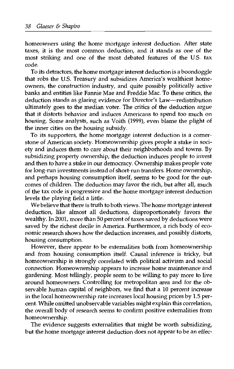
tive means of subsidizing ownership.

While the deduction appears to

increase the amount spent on housing, it also appears to have almost no

effect on the homeownership rate. The best evidence for this claim is the

simple time series shown in Figure 1. Since 1965, the inflation rate has

soared and collapsed, causing the subsidy to homeownership similarly

to rise and fall [our formula for the subsidy is based on Poterba (1992)].

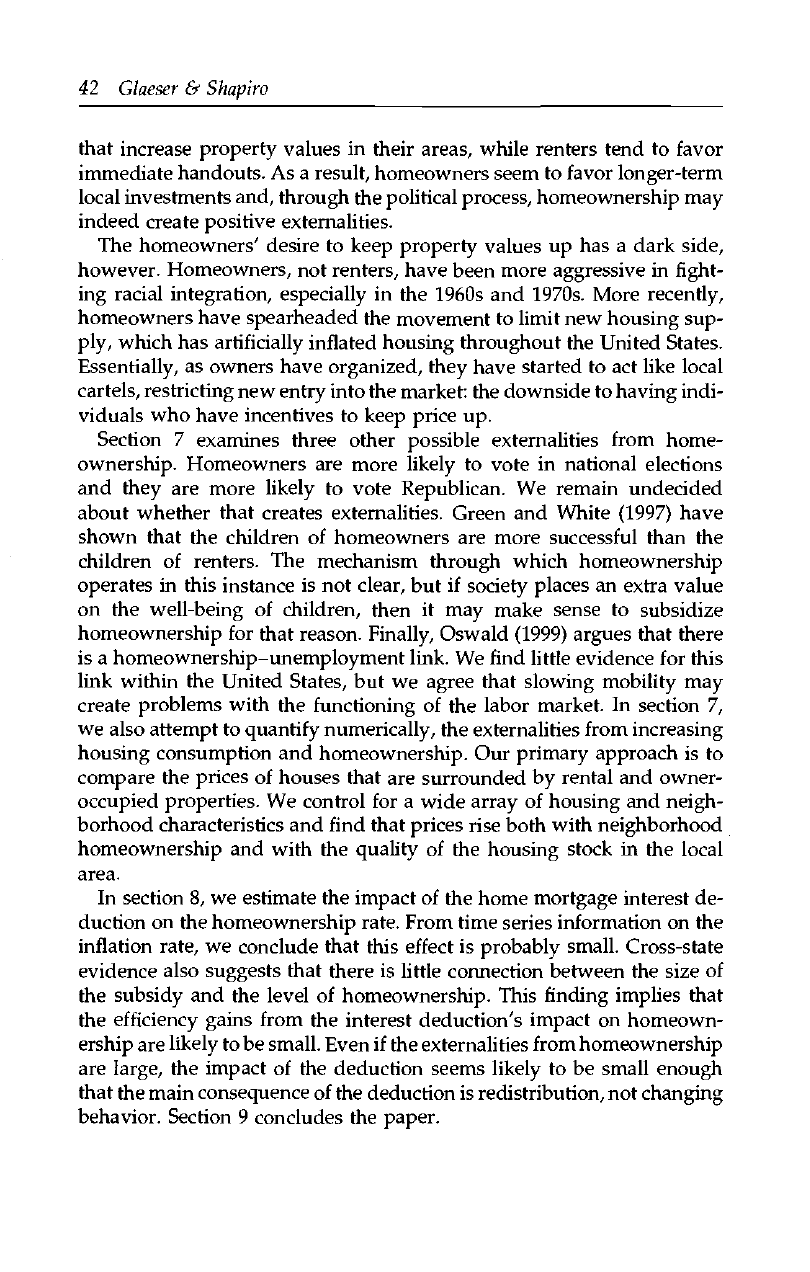
As Figure 2 also shows, changes in the tax code have caused itemization

rates to rise and fall. If the tax code affected homeownership powerfully,

we might expect a relationship between itemization rates and homeown-

ership, but as Figure 2 shows, there is no such relationship. Since the

1960s, the homeownership rate has barely budged, staying within a fixed

band between 63 and 68 percent. The changes in the itemization rate that

have occurred seem more related to the suburbanization of the economy

than to the subsidy created by the deduction.

When we speak of the home mortgage interest deduction as a subsidy, we mean to com-

pare it to a benchmark of our current tax system absent the deduction, rather than to alterna-

tive tax policies such as a consumption tax.

Glaeser

Shapiro

FIGURE 2. Trends in Itemization, 1965-2000

—©— Percentage itemizing —*— Homeownership rate

1965 1970 1975 1980 1985 1990 1995 2000

Year

* Series is percentage of all federal tax returns itemizing deductions. Data from www.irs.gov.

This relative invariance of the homeownership rate shouldn't surprise

us.

Homeownership is almost perfectly linked with the type of housing

structure. People living in single-family detached units usually own and

people who live in multifamily units rent. Because this stock of housing

is relatively fixed in the short run, we shouldn't expect much of a response

in the homeownership rate to any short-run fluctuations. In the long run

though, the power of the home mortgage interest deduction to affect

homeownership is also likely to be small. The groups that are really on

the homeownership margin (the poor and the young) rarely use the de-

duction, even when they are owners. Thus, the deduction is unlikely to

influence the homeownership rate. The limited impact of the deduction

on homeownership means that there is little distortion of the ownership

margin due to the home mortgage interest deduction and, as such, the

deduction serves mainly to increase housing consumption and to change

the progressiveness of the tax code.

1.1 Plan of the Paper

In section 2 of this paper, we review basic facts about itemization, the

home mortgage interest deduction, and homeownership. First, we review

While some authors attack the deduction because it makes the income tax code less progres-

sive,

it is not obvious to us that making the tax code more progressive is a beneficial goal.

The Benefits of the Home Mortgage Interest Deduction 41

the distribution of itemization throughout the population. Even among

homeowners, itemization is extremely rare in the bottom deciles of the

population. As a result, the home mortgage interest deduction creates tax

savings overwhelmingly for the top deciles of the income distribution.

Second, we review the correlates of homeowner

ship.

Homeownership

is particularly correlated with housing structure. People who live in

multifamily dwellings rent—people who live in single-family detached

houses own. We believe that this situation stems from agency problems

related to home maintenance. Housing structure itself is very highly cor-

related with age and position in the life cycle. An overwhelmingly large

share of nonpoor Americans who are married live in single-family houses.

Together, these facts mean that the home mortgage interest deduction

affects a subset of the population that almost never rents.

In section 3 of the paper, we review the economics of the home mort-

gage interest deduction. This deduction creates an incentive both to

consume more housing and to own. In section 4, we consider evidence

on possible externalities from housing consumption and home quality,

rather than homeownership

itself.

In section 5, we turn to the theory be-

hind the social benefits of homeownership. There are three ways that

homeownership might create externalities. First, homeowners might take

better care of their property, which might create externalities. Second,

because they own an asset whose value is tied to the quality of their com-

munity, homeowners might work harder to make their community pleas-

ant. Third, homeowners face higher mobility costs, which might induce

them to invest more in their community. We find evidence for all of these

channels.

In section 6, we look at homeownership and neighborhood externali-

ties.

First, and most obviously, is maintenance/gardening. While it

sounds trivial, there is little doubt that owners spend more time main-

taining their houses and gardens, and panel evidence suggests that this

characteristic is not just the result of different people being homeown-

ers—people take better care of their houses when they own. This effect

appears to create at least 50 percent of any spillovers from homeown-

ership. There is also evidence suggesting that homeowners are more in-

volved in local social groups and are more likely to work to solve local

problems. In section 6, we also consider the consequences of homeown-

ership for local politics. DiPasquale and Glaeser (1999) showed that home-

owners are more likely to vote locally. DiPasquale and Glaeser (1998)

and Monroe (2001) showed that municipalities with homeowners are par-

ticularly likely to spend more on schools and streets and less on social

welfare and hospitals. Theory predicts that homeowners favor policies

42 Glaeser & Shapiro

that increase property values in their areas, while renters tend to favor

immediate handouts. As a result, homeowners seem to favor longer-term

local investments and, through the political process, homeownership may

indeed create positive externalities.

The homeowners' desire to keep property values up has a dark side,

however. Homeowners, not renters, have been more aggressive in fight-

ing racial integration, especially in the 1960s and 1970s. More recently,

homeowners have spearheaded the movement to limit new housing sup-

ply, which has artificially inflated housing throughout the United States.

Essentially, as owners have organized, they have started to act like local

cartels, restricting new entry into the market: the downside to having indi-

viduals who have incentives to keep price up.

Section 7 examines three other possible externalities from home-

ownership. Homeowners are more likely to vote in national elections

and they are more likely to vote Republican. We remain undecided

about whether that creates externalities. Green and White (1997) have

shown that the children of homeowners are more successful than the

children of renters. The mechanism through which homeownership

operates in this instance is not clear, but if society places an extra value

on the well-being of children, then it may make sense to subsidize

homeownership for that reason. Finally, Oswald (1999) argues that there

is a homeownership-unemployment link. We find little evidence for this

link within the United States, but we agree that slowing mobility may

create problems with the functioning of the labor market. In section 7,

we also attempt to quantify numerically, the externalities from increasing

housing consumption and homeownership. Our primary approach is to

compare the prices of houses that are surrounded by rental and owner-

occupied properties. We control for a wide array of housing and neigh-

borhood characteristics and find that prices rise both with neighborhood

homeownership and with the quality of the housing stock in the local

area.

In section 8, we estimate the impact of the home mortgage interest de-

duction on the homeownership rate. From time series information on the

inflation rate, we conclude that this effect is probably small. Cross-state

evidence also suggests that there is little connection between the size of

the subsidy and the level of homeownership. This finding implies that

the efficiency gains from the interest deduction's impact on homeown-

ership are likely to be small. Even if the externalities from homeownership

are large, the impact of the deduction seems likely to be small enough

that the main consequence of the deduction is redistribution, not changing

behavior. Section 9 concludes the paper.

The Benefits of the Home Mortgage Interest Deduction 43

BASIC FACTS ABOUT ITEMIZATION

AND HOUSING

Figure 2 shows the path of itemization over time in the United States since

1965.

In 1950, only 19.4 percent of Americans itemized. Over the 1950's,

this share doubled to 41.1 percent and hit a peak of 47.6 percent in 1970.

Responding, presumably, to the Tax Reform Act of 1969, the share of re-

turns that included itemization fell to 34.8 percent by 1972. Between 1972

and 1986, the share of returns that included itemization rose again, to a

peak of 39.1 percent in 1986. Since the 1986 Tax Reform Act, the share of

returns with itemization has been steady: around 30 percent.

The 30 percent of the population who itemize are distributed dispropor-

tionately among the upper income brackets. Table 1 shows the share of

itemizers (and the share of total itemized income) by income decile based

on information from the 1998 Survey of Consumer Finances. Slightly over

one-half of the itemizers are in the top two income deciles. More than 50

percent of the overall itemized income is in the top decile alone. The poor-

est 40 percent of the population contains only 5 percent of the itemizers,

and they are responsible for 3.5 percent of the total itemized income.

Table 1 also shows itemization rates for homeowners and renters by

income bracket. The table makes clear that, among the poorest Americans,

itemization is very rare for either owners or renters. On average, 12.9

percent of homeowners in the bottom 40 percent of the income distribu-

tion itemize. On the other hand, almost 50 percent of people in the top

decile itemize, whether they are owners or not. These facts are not surpris-

ing, but they illustrate the extent to which the home mortgage interest

deduction is targeted toward wealthier Americans.

But homeownership is high even among the rich who don't itemize. In

the top income decile, the share of homeownership among nonitemizers

is still over 75 percent. In Table 2, we look at the relationship between

income and homeownership again using the Survey of Consumer Fi-

nances. In regression (1), we find that the marginal effect of the log of

income on the probability of being a homeowner is .19. In regression (2),

this coefficient falls to .13 when we control for itemization. Income still

strongly determines homeownership. Because itemization is itself a func-

tion of homeownership, controlling for itemization is problematic, so

these results are merely descriptive. In regression (3), we control for build-

ing structure and find that the coefficient on income remains at .13.

As the results in column (3) of Table 2 illustrate, homeownership de-

pends to a considerable degree on taste for structure. To explore this is-

sue further, we split structure type into four categories: single-family

44 Glaeser

Shapiro

•p

CL,

.•a

WONODHHOOOrlO-*

fN^DvqtNCNt>.fNlN

(NlO

O H (N ^

5 xi

0.1917

(0.0027)

20,215

0.1317

(0.0029)

0.2711

(0.0068)

20,215

0.1316

(0.0036)

0.1900

(0.0083)

0.1229

(0.0217)

-0.4019

(0.0239)

0.0948

(0.0252)

18,525

The Benefits of the Home Mortgage Interest Deduction 45

TABLE 2

Homeownership and Income*

(1) (2) (3)

Log(income)

Itemizer

Single-family detached home

Home in multi-unit structure

Mobile home

Observations

* Regressions are from authors' calculations based on the Survey of Consumer Finances, 1998. Coefficients

are marginal effects from probit models. All coefficients are significant at the 1 percent level.

detached, which represents 59 percent of the housing stock of the United

States; single-unit attached, which represents 6 percent of the housing

stock; multiunit attached, which represents 30 percent; and mobile homes,

which represent 5 percent of the housing stock. Eighty-five and one-half

percent of people living in single family detached homes are owners, and

85.9 percent of people living in multifamily units are renters. People living

in mobile homes generally also own (79.6 percent). The only category that

is clearly mixed is single-family attached homes, where 53.2 percent own.

Another way of thinking about this relationship is that the correlation

between living in a single-family detached home (or mobile home) and

owning is 58 percent. At the city level (among cities with more than 25,000

inhabitants in 1990), the correlation is even higher—73 percent. Figure 3

shows the relationship between owning and living in single-family de-

tached houses across cities in the United States with more than 25,000

inhabitants. There are few facts in urban economics as reliable as the fact

that people in multifamily units overwhelmingly rent and people in

single-family units overwhelmingly own.

The most convincing theory to explain this fact is that the agency prob-

lems with home maintenance lead to having exactly one owner for each

building, as suggested by Henderson and Ioannides (1983) and Kanemoto

(1990).

The literature on home maintenance (DiPasquale and Glaeser,

1999;

Shilling, Sirmans, and Dombrow,

1991;

and Galster, 1983) documents

that in single-family units, renters take worse care of their homes than

do owners, and that rental homes depreciate faster. This finding is unsur-

prising. Owners face strong incentives to maintain their property; renters

46 Glaeser & Shapiro

FIGURE 3. Homeownership and Structure'

100

-occupiec

! owneritagercer

o 8 o °

Percentage single-family detached housing

100

* Graph shows percentage of housing that is owner-occupied and percentage of housing that is single-

family detached in 1990 for places containing 25,000 people or more. Data from the City and

County Data

Book,

1994.

face much weaker incentives. The agency problems involved with renting

single-family detached homes (or mobile homes) make it natural for these

structures generally to be owner-occupied.

However, the major maintenance problems in multi-unit dwellings are

all building-, not unit-, specific. A large structure has one boiler, one

roof,

and one electrical system. These featers are best maintained by a single

owner. Several owners jointly responsible for maintaining these common

building attributes, creates a huge free-rider problem. As a result, it makes

sense for multi-unit dwellings to be rental units with a single owner.

There is no concrete evidence on the management costs involved in coop-

erative apartment buildings, but anecdotal evidence suggests that the

agency problems are immense.

Large amounts of tenant time are fre-

quently spent trying to manage these large structures, and generally this

type of management rarely seems to be efficient. The maintenance prob-

lems appear to be building specific, so agency theory would suggest the

One treasurer of a New York City cooperative apartment building describes two primary

sources of waste. First, cooperative apartment owners lack the specialized expertise needed for

large-scale technical problems and complex legal issues. Second, board meetings often devolve

into lengthy debates over unclear property rights and get mired in interpersonal conflict.

The Benefits of the Home Mortgage Interest Deduction 47

simple rule—one building, one owner—and this is what we generally see

in the United States.

This strong relationship between building structure and ownership

means that viewing homeownership solely as a portfolio decision is in-

valid. The homeownership decision generally involves a simultaneous

decision about structure. Subsidizing homeownership will have only

modest short-term effects because the building structure is relatively

fixed. We think that the connection between ownership and structure type

also suggests that subsidizing homeownership may have only modest

long-term effects as well because, in many cases, it would require a very

large subsidy to prompt a well-to-do family of five to live in a multi-unit

building. By the same token, multi-unit areas are unlikely to become filled

with homeowners. Indeed, the massive distortions of rent control only

managed to increase the homeownership rate of New York City—which

is filled with multifamily dwellings—to 30 percent. To us, this situation

implies that the ability to shift multifamily units to cooperative or condo-

minium status has limits.

TAXES AND HOUSING

The tax treatment of homes potentially changes behavior along two mar-

gins:

the decision to own or rent and the decision of how much housing

to consume. The home mortgage interest deduction both induces individ-

uals to consume more housing and to own the housing that they do con-

sume. In this discussion, we focus on the impact of that deduction, but

other aspects of the tax code (and government policy more broadly) also

affect the homeownership decision.

For example, much literature emphasizes the pro-renter aspects of some

areas of the tax code (see, for example, Gordon, Hines, and Summers,

1987).

In particular, the accelerated depreciation schedule for landlords

tends to support the construction of structures relative to other forms of

capital. This feature of the tax code tends to increase the consumption of

rental housing (just like the home mortgage interest deduction). Unlike

the home mortgage interest deduction, it is not as targeted to wealthier

Americans because accelerated depreciation applies to almost all rental

units.

This paper will not focus on these issues and will pay more atten-

tion instead to the home mortgage interest deduction alone.

There are substantial cross-national differences in ownership patterns that might lead one

to doubt the universal applicability of that rule. Proper analysis of these differences lies

beyond the scope of this paper, but we certainly accept the point that large enough policy

differences toward housing can indeed turn apartment dwellers into owners or people in

single-family houses into renters.

48 Glaeser & Shapiro

Because there are two distinct margins that are affected by the home

mortgage interest deduction, it makes sense to separate discussion of tax

reform into two separate questions. First, should the tax system continue

to subsidize the level of housing consumption? (Are there social benefits

from building bigger homes?) Second, should the tax system continue to

subsidize owning relative to renting? (Do we want to encourage Ameri-

cans to own property?)

The efficiency arguments for subsidizing either the level of housing

consumption or homeownership rely on the existence of externalities. The

case against the subsidy focuses on the distortions created by the tax code.

Of course, there may also be desirable or undesirable distribution conse-

quences of transferring from renters to owners and transferring from peo-

ple who consume little housing to people who consume more expensive

housing. It is also possible that there are negative externalities associated

with either ownership or the level of housing consumption.

The literature on the home mortgage interest deduction is oddly bifur-

cated. The authors who focus on the costs of the deduction focus entirely

on the amount of housing consumed. Aaron (1972), Rosen (1979, 1985),

Poterba (1984,1992), and Mills (1987) are but a small sample of the authors

who have looked at the social costs of overconsuming housing due to the

home mortgage interest deduction. The authors who look at the possible

benefits of the deduction look only at the benefits of ownership. This

much smaller group includes DiPasquale and Glaeser (1999), Green and

White (1997), and Rossi and Weber (1996). None of their papers even men-

tions the possible costs of overconsuming housing.

We begin with a brief formal analysis, following Poterba (1992), on the

home mortgage interest deduction and the housing capital gains exemp-

tion on the price of housing. To permit this analysis, we look at the impact

of tax policy on the steady-state cost of housing, and we assume (as does

Poterba) that the price of housing is rising deterministically with the level

of inflation. We let n denote the inflation rate, i denote the real interest rate,

x denote the federal income tax rate, and x

denote the local (deductible)

property tax rate. The quantity of housing is denoted as H, and the price

per unit of housing is P

. We assume that the standard deduction is D.

Our one substantive difference from Poterba's model is that we assume

the depreciation and maintenance costs differ for renters and owners. This

assumption is meant to capture the agency costs involved in renting, or

the problems involved in coordinating multiple owners of a multi-unit

dwelling. We denote the total maintenance and depreciation costs as d

for renters and d

for owners. Following our previous discussion, we as-

sume that d

is greater than d

for single-unit dwellings and that d

greater than d

for multi-unit dwellings.

The Benefits of the Home Mortgage Interest Deduction 49

Free entry of landlords (that is, a zero profit condition) implies that the

free-market rent for a unit of housing equals (i + x

+ d

, in after-tax

dollars. For owners who itemize, the per unit cost of housing equals (i +

)(l

—

x) + d

—

ITI)PH-

For owners who don't itemize, the per unit cost

of housing equals (i + T

+ d

~ T0(f + n))P

where 6 refers to the fraction

of the house that is financed with the owners' capital (as opposed to debt).

Nonitemizers (as opposed to itemizers) face tax-created incentives to put

everything into their home because the capital gains in that asset are not

taxed. The home mortgage thus provides an incentive for owners who

don't itemize to invest more in housing (at least relative to renters). This

incentive is much higher for individuals who itemize and higher too for

individuals who face high tax rates.

One way to think about this incentive that we will use later is the per-

centage decrease in the price of housing created by the tax code relative

to a nondurable good with a price of 1. The percentage reduction in the

price of owned housing created by the federal tax code equals

+ K +

(i + x

)(l - x) + d

- xn

If we assume that the real interest rate is 2 percent, the nominal interest

rate is 6 percent, the local property tax rate is 1 percent, the depreciation

and maintenance cost is 3 percent ($3,000 per year on a $100,000 home),

and the federal tax rate is 25 percent, then this number equals 41 percent.

If depreciation and maintenance are as high as 5 percent, then this number

would fall to 28 percent, which is still quite sizable. For nonitemizers, we

have financed 80 percent of their house with their own equity, and the

subsidy equals 7 percent of the cost of the home if maintenance is 3 per-

cent of total costs.

The benefit from owning (as opposed to renting) a house of fixed size

equals (i + n + x

)x + d

—

) per dollar spent on housing if the individ-

ual itemizes when he or she is both an owner and a renter. If the individ-

ual itemizes only when he or she owns, the incentive to own (again per

dollar spent on housing) equals (i + n + x

)x + d

—

TD/P

the individual doesn't itemize in either case, then the incentive to own

relative to the cost of housing equals x0(f + n) + d

— d

Table 3 shows the magnitude of these three tax-related subsidy values

for different parameter values. The tax-related subsidies exclude the

depreciation elements from each expression, and they equal (z + n + x

)x,

(i + n + x

)x -

%D/P

and xG(z + 7i) for the three always owners,

sometimes owners, and never owner, respectively. Poterba (1984) empha-

50 Glaeser & Shapiro

Real

interest,

Inflation,

TABLE 3

Subsidy per Dollar for Itemizers

Property

tax, x

Federal

tax, x

25%

Subsidy to

when

Always

homeownership,

itemizing

When

own

Never

0.30%

0.25

0.35

0.30

0.25

0.35

sized the powerful effect that inflation has on the incentive to consume

more housing—but the incentive that inflation creates to own homes is

just as strong. As the table shows, when the inflation rate rises, the subsidy

(at least for the itemizers) rises significantly. For individuals who don't

itemize in either case, the subsidy tends to be small. For example, as the

table shows, a less wealthy individual who has financed 80 percent of the

value of the house with debt and who faces a marginal federal tax of 25

percent and a nominal interest rate of 7 percent, the value of T0(z + n)

equals .35 percent.

It certainly wouldn't surprise us if the difference between d

and d

2 percent (positive for single-family dwellings and negative for multi-unit

homes). In this case, the depreciation-related incentive to own (or rent)

will swamp the tax-related benefits of owning for individuals who don't

itemize in either case. This situation may explain why changes in the tax

subsidy do not seem to change the homeownership rate.

The tax code creates incentives both to consume more housing and for

people to own their homes. These incentives are focused on wealthier

people who are likely to itemize. Among nonitemizers, the incentive to

own increases only for those buyers who pay for a significant fraction of

their own homes. We will return to the impact of changes in the incentive

to own on the homeownership rate, but first we will discuss the incentive

to overconsume, which has received a much larger share of academic

attention.

SUBSIDIZING HOUSING CONSUMPTION

The case for subsidizing housing consumption is based on a desire either

to redistribute income to people who buy a lot of housing or to encourage

The Benefits of the Home Mortgage Interest Deduction 51

people to consume more housing. We have little to say about the benefit

of redistributing to those who consume a lot of housing, so we will focus

on the benefits and costs of inducing greater consumption of housing.

The usual justification for a subsidy to something like housing is based

on claims about externalities, i.e., social benefits from housing that are

not internalized by the individuals themselves. By this reasoning, people

generally buy too little housing, and the home mortgage interest deduc-

tion induces them to step up to the plate and consume the size of houses

that they should consume if they internalized all the benefits that more

expensive housing creates for society.

Three main externalities might come from housing consumption. First,

sufficiently poor housing could spread disease and fire. Indeed, through-

out most of history, government intervention in the housing market has

been motivated mainly by a desire to impose minimum standards on

housing to stem the flow of infectious diseases and to reduce the threat

of widespread urban fires. Second, better housing might create aesthetic

amenities that bring pleasure to neighbors and passersby. Third, housing

might benefit children. If the government, in general, cares more about

children relative to parents, and parents care about children relative to

themselves, then there is a case for subsidizing commodities that specifi-

cally benefit children.

The first externality is probably at best minimally relevant in twenty-

first-century America, at least outside the poorest areas. Most people are

living in well-ventilated, relatively fire-resistant homes. Outside the bot-

tom quartile of society, Americans live in good homes. Fire and safety

codes,

which are often fairly draconian, appear to be much more effective

in limiting the dangers from fire than a blanket home mortgage interest

deduction.

Given that health and fire externalities are very rare except among the

poorest Americans, the home mortgage interest deduction is poorly de-

signed to correct those externalities. The American Housing Survey

(AHS) also illustrates that wealthier Americans, i.e., Americans in the top

half of the income distribution, are unlikely to live in either crowded or

dangerous housing. For example, 95 percent of the top 70 percent of the

income distribution live in homes with more than 228 square feet per

capita. This number may seem small relative to the newer McMansions,

but it is higher than the median square footage per capita in London,

Paris,

or Rome, and it certainly is not crowded by any standard. The AHS

also tells us that home problems, such as leaks and rats, are very rare

among any but the poorest Americans. Indeed, in the entire AHS, more

than 40 percent of the housing problems occur in the poorest 25 percent

of the population and less than 15 percent of this population itemizes,

52 Glaeser & Shapiro

even if they own. The home mortgage interest deduction doesn't provide

incentives for the population groups that are really at risk of consuming

substandard housing.

A second externality is aesthetic—perhaps people enjoy looking at fan-

cier homes and, as a result, people should be induced to consume big

houses. In principle, the externality from fancy homes might be either

positive or negative. Living around nicer homes might provide a positive

experience. On the other hand, particularly fancy homes might incite envy

and actually create negative utility. Thus the externality from home qual-

ity is theoretically, at least, ambiguous.

One could easily argue that aesthetic externalities are not really a fit

subject for federal government policy. After all, aesthetic tastes are quite

heterogeneous, and it makes little sense to try to influence these tastes

with federal tax policy. Indeed, zoning and land-use controls appear to be

much more appropriate instruments for internalizing visual externalities.

Localities appear to be quite effective (perhaps too much so) at regulating

the appearance of their homes.

It seems sensible, however, to test whether there is evidence for exter-

nalities from housing consumption. If the evidence suggests large exter-

nalities, particularly among the rich, then there may be a case for

subsidizing the housing consumption of this group through the home

mortgage interest deduction.

The standard approach to quantifying these forms of externalities is to

see whether people pay more for homes in places where other homes

are nicer, i.e., the hedonic approach. In this approach, for each house we

estimate

log(price) = a X attributes + b X neighboring housing quality (1)

+ c X other controls

There are several standard problems with hedonic regressions of this

form. Measured neighborhood home quality is likely to be correlated with

unobserved attributes of the house and neighborhood that also affect the

value of the house. This correlation is likely to bias our estimates upward.

The standard criticisms of hedonic estimation (Epple, 1987) also apply.

Nonetheless, in Table 4, we proceed with a hedonic estimate of the spill-

overs from living around nicer homes. We use the 1993 neighborhood

survey from the American Housing Survey. This survey is a variant of

the standard housing survey with detailed information on housing qual-

ity. The advantage of this neighborhood survey is that the AHS gathers

information on the 10 closest neighbors. We have information on the char-

The Benefits of the Home Mortgage Interest Deduction 53

acteristics of the neighbors' housing (and their own demographics). This

information can, in principle at least, help us to identify the magnitude

of some spillovers.

Housing prices are self-reported and this feature may create biases.

However, Goodman and Ittner (1992) find that self-reported housing val-

ues generally overstate true values, but that this overstatement is fairly

orthogonal to other features of the house. The bias from self-reported as

opposed to market values is thus not likely to confound our results too

much.

In all of our regressions, we include a large array of standard house

characteristics that are standard in the literature. We are not focused on

the value of the coefficients on these attributes, but rather we see them

as a control. We also include the average education in the 10-house clus-

ter. This control is meant to control for the average human capital level

of community. The estimates in regressions (l)-(3) of Table 4 seem quite

sensible and suggest that housing prices increase by slightly more than

3 percent with each year of schooling in the neighborhood.

In regression (1), we include three measures of average neighborhood

housing quality: mean lot size, mean unit size, and mean number of hous-

ing problems. These averages are based on the housing characteristics of

the other 9 units in the 10-unit cluster. We use a value of 0 for the lot size

of apartments. The housing problems measure is the AHS index measure

for capturing the presence of substandard housing. At the house level,

each new problem is associated with a 9 percent lower housing value.

Both the neighborhood lot size and the unit size coefficients go in the

wrong direction—being around bigger homes reduces housing values.

We interpret these coefficients as showing the omitted variables problems

in these regressions. Presumably, people buy bigger lots in areas that are

cheaper, and so we shouldn't be surprised to see the negative coefficient.

Only the mean number of problems coefficient goes in the expected direc-

tion, and it does suggest that houses are cheaper, holding their character-

istics constant, if their neighbors have more housing problems. Still, the

omitted variables problems continue to make interpretation of this coeffi-

cient difficult.

In regression (2), we include a composite housing quality measure by

using the hedonic parameters estimating a basic housing hedonic. To

make averaging sensible, we regress the housing price itself (not its loga-

rithm) on housing characteristics. We use these estimated coefficients to

create a predicted housing value for each apartment. We take the average

of the predicted house value for the other nine houses in the cluster and

log that average value to get an elasticity. These results are robust to alter-

native averaging procedures (i.e., taking the average of a log estimate).

54 Glaeser & Shapiro

_«

•6

12:

T-H

IN CN|

tN (N 00

Hino^irj

q oq

H CN

T—I

IN CO

T-H

^O 1—I

T—I

CN T-H ^H

r-J

d d d d d

IN TJ<

O O

tNCO

CNOLfNCOr-l

rH^OOCOCNO^OO

COOOOOOCNONlN

pppppOCNO

00^00,00^00

I I "

ling

rs of scho

Mean

size

Mean

t size

uniMean

blem

number of pi

Mean

price

Log

redic

log mean

third

Spline

Bott

thirddieMid

thi

Top

price

Log m

rice:

log mean

Spline

third

Bott

third

dieMid

thi

Top

ons

Obser

The Benefits of the Home Mortgage Interest Deduction

NHinMN

OOOOOO

OOOOOOOOOOO

^ I

id,

o'ooo'oo

i o i

oooo'o'oo'o'o'o'o

I o I

oo'o

S-

00,00^00,

o,oo,od,oo,o'o,oo,

o,'

'o,22,^

^fOm

00,00,00,

0,00,00,00,00,00,

OOOOOO

OOOOOOOOOOO

oMscoH

OCNOOO

^^-1?Oppl§^^

I >_• *>

•_/

V1 W

—.

\^S

—^

>_^ I. N V^^

\_^ ^_^

>«^ v_^ ^

V_/

-_^

-»_/

—.

•^B/

00,00,00,

0,00,00,00,00,00,

cond

<ri

typ

ating

^QJ

pr<

ions

.SP

CL,

56 Glaeser & Shapiro

We find an overall coefficient of .086, which means that a 1 percent in-

crease in average housing quality in the neighborhood is associated with

an 8.6 percent increase in the value of the house. This coefficient would

imply an optimal subsidy of 8.6 percent to the price of housing (which

is much less than the subsidy that actually exists for itemizers).

In regression (3), we estimate a spline in this average predicted value

parameter. This estimate enables us to check whether the impact of the

average value is different for poorer neighborhoods or for richer neigh-

borhoods. We estimate the impact of average predicted housing values

with two breaks, corresponding to the thirty-third and sixty-sixth percen-

tile of the average home price distribution. Surprisingly, the strongest co-

efficient occurs for the top third of the housing price distribution. There

is no effect of housing quality in the bottom third. The coefficient for the

middle third is .27, and the coefficient for the top third is .4. In principle,

these estimates could justify exactly the subsidy that we see in practice:

a generous housing consumption subsidy oriented toward the top of the

income distribution. Still, we believe that these results are sufficiently rid-

dled with omitted variables problems that we would be loath to accept

them without more

proof.

Finally, in regression (4), we use the actual prices of one's neighbors to

estimate the average housing quality in the neighborhood. This variable

has the advantage of capturing unobserved housing attributes. In other

words, if the American Housing Survey does not adequately measure some

housing attributes (say, the aesthetic qualities of the house), then these attri-

butes will still be included in the price. However, this variable has the disad-

vantage of incorporating omitted, neighborhood level characteristics,

which would induce a spurious correlation between the dependent housing

price and the housing prices of the neighboring houses.

Overall, we find a large effect from the average housing price of the

neighbors. The estimated coefficient is .89. In regression (5), we perform

the same spline as in regression (4), but here we use actual housing prices

instead of predicted housing prices. As in the previous regression, we

find that the impact of neighborhood housing price is the same at all hous-

ing quality levels. We are particularly suspicious about these results be-

cause unobserved factors that make houses expensive are likely to affect

the entire neighborhood.

Overall, these results suggest that there may well be externalities in-

volved in consuming more housing. Still, the home mortgage interest de-

duction subsidizes housing consumption beyond the level that would be

justified by our preferred estimates in regression (2).

Finally, it is possible that there is an intergenerational externality re-

lated to housing consumption. In principle, larger, more comfortable

The Benefits of the Home Mortgage Interest Deduction 57

homes may benefit children. If the government cares more about children

(relative to parents) than parents do, then it may make sense to subsidize

homeownership.

We don't know of any evidence that documents the

impact of extra space on the outcomes (or happiness) of children, but we

do know that housing consumption and children are clearly comple-

ments. On average, the amount of interior space rises by 48 square feet per

additional child in the American Housing Survey. This complementarity

makes it possible at least that subsidizing housing may yield benefits for

children. Of course, in most cases the disadvantaged children that we are

most concerned about helping will not be affected by the home mortgage

interest deduction.

The complementarity between housing consumption and children

means that the mortgage interest deduction may also have an impact on

fertility. If larger homes make big families possible, then subsidizing

housing will be desirable if the government desires to subsidize fertility.

Indeed, elsewhere we have shown that there is at least some relationship

between fertility and floor area per capita across countries. While this

correlation can be due to reverse causality or omitted variables, it is still

suggestive and at least raises the possibility that the U.S. government's

pro-housing policies may play some role in supporting high American

fertility. Of course, this impact on fertility is only desirable if we want to

subsidize fertility to begin with, a goal that is far from obvious.

4.1 Negative Effects of Subsidizing Housing

Consumption

Numerous papers have talked about the welfare losses from subsidizing

housing consumption in the absence of externalities. These papers have

taken the straightforward economic view that distorting consumption cre-

ates welfare losses relative to an outcome where prices reflect social costs.

However, these losses will increase if there are negative, not positive, ex-

ternalities from certain types of housing consumption. Here, we mention

briefly the possible negative externalities related to subsidizing housing

consumption through the home mortgage interest deduction.

Voith (1999) has argued that subsidizing housing consumption may

indeed be hurting our inner cities. His argument is that, by encouraging

more housing consumption, the home mortgage interest deduction en-

courages people to leave small city apartments to consume larger places

on the fringe of the city. This flight from the city might itself impose nega-

tive social costs on the people who remain in the city.

If a parent values his or her child's utility almost as much as his or her own, but the

government values both equally (even if it doesn't care much about either one of them),

then the government should act to create incentives for transfers from parent to child.

58 Glaeser & Shapiro

More generally, the home mortgage interest deduction may create neg-

ative effects by disproportionately encouraging spending on housing

among the wealthy, and not among the poor. To the extent to which

spending is limited to structure, this unequal incentive seems unlikely to

cause social problems. However, a significant amount of spending in the

expensive areas of the country is on land, or community amenities, not

on structure (see Glaeser and Gyourko, 2002). Thus, the home mortgage

interest deduction encourages the rich to spend more on community

attributes.

Again, this situation is not necessarily problematic if community attri-

butes are innate items like access to the seacoast, but it is a problem if

the primary community attribute is the average income, or human capital

level, of the community. If we encourage the rich to buy more, then we

encourage the rich to live in particularly high-income communities. In

essence then, the home mortgage interest deduction acts to increase segre-

gation by income. By creating incentives for the rich to spend more on

housing, the home mortgage interest deduction creates incentives for the

rich to live in better neighborhoods, which means that the rich will tend

to segregate more.

To make this concrete, consider the following simple algebraic example.

Consider a world with N rich people and N poor people living in two

communities, each of size N. All houses are identical, except that people

get utility from the percentage of rich people in the community equal

to a X r, where r is the percentage of the community that is rich and a is

an individual specific parameter that is districted on the interval: [a

—

+ e] for the rich and [a

—

e, a

+ e] and for the poor, where oc

> a

The equilibrium condition for this model is that the difference in housing

prices between the two neighborhoods must offset exactly the utility gains

from being in a neighborhood with more rich people. In the absence of

subsidized housing, there will be one rich community with a proportion

of rich residents equal to

- a

.D i

4£

and a poor community with a proportion of its residents that are rich

equal to

_ a

- cc

4£

If the tax code subsidizes housing consumption for the rich (and not the

poor) so that they pay only 1

—

s of any housing costs, then in the new

The Benefits of the Home Mortgage Interest Deduction 59

equilibrium, the rich community will have a proportion of rich residents

equal to

5 +

- (1 - s)a

2(2 - s)e

and the poor community will have a proportion of rich residents equal

_ a

- (1 - s)a

2(2 - s)£

The degree of segregation (i.e., the share of the rich who live in the rich

community) rises with the degree of subsidization. Any policy that makes

it cheaper for the rich (relative to the poor) to live in the more expensive

neighborhood will tend to increase the degree of segregation in society.

Conversely, a policy that disproportionately subsidizes the housing con-

sumption of the poor (perhaps Section 8 vouchers) would act to decrease

income segregation.

Cutler and Glaeser (1997) argue that black-white segregation is quite

harmful to African-Americans. If subsidizing housing consumption abets

this segregation, then it will create negative externalities for African-

Americans. Because we do not have meaningful estimates of the impact

of the subsidy on the level of segregation, it is impossible at this time to

calculate the welfare costs from this aspect of housing subsidy. Still, we

highlight this potential negative impact of the home mortgage interest

deduction as a topic for future research.

5. THE EXTERNALITIES FROM OWNERSHIP

We now switch from considering the housing consumption margin to

considering the ownership margin. The bulk of the discussion about the

benefits of the home mortgage interest deduction has focused on this mar-

gin and the externalities from homeownership. At this point, we address

first the issue of whether there are externalities from homeownership,

and if so, how important they are. Then we turn to the issue of whether

the home mortgage interest deduction does a good job of promoting

homeownership.

Indeed, Katz, Kling, and Liebman (2001) find that voucher recipients tend to use their

vouchers to move to low-poverty neighborhoods, even when there is nothing explicit about

the voucher that subsidizes nonpoor neighborhoods.

60 Glaeser & Shapiro

The economics literature points to three reasons why homeownership

might create externalities. First, homeowners own an asset whose value

is tied to the strength of their community. Thus, they have an incentive

to act (and vote) for policies and practices that will make their community

more attractive. This civic participation may take the form of community

activism or contributions to public goods. Of course, free-rider problems

still exist, but the property stake in the community creates at least a small

incentive to keep the community strong.

This scenario becomes particularly clear in the case of elections. Home-

owners tend to prefer government actions that promote the value of their

property. In many cases, these actions may be long-term investments that

raise the long-term prospects of the community. Because housing is a

long-lived asset, it will incorporate expectations about the results of gov-

ernment investment, and owners will reap benefits from long-term gov-

ernment incentives.

Conversely, renters have no financial stake in strengthening the com-

munity and they can even lose from investments that strengthen the com-

munity because rents are not fixed. If these investments are sufficiently

attractive to outsiders, then they will raise rents more than they raise the

utility of the renters directly and the renters may lose. Thus, renters are

likely to prefer direct government handouts that come to them, while

owners will be more likely to trade off such handouts for investments in

the community. (The algebra of this argument is given in DiPasquale and

Glaeser, 1999.)

The political interest of homeowners has a dark side. Owners face in-

centives to raise house prices by any means possible. In some cases, im-

proving the community is a natural means of raising prices. In other cases,

stopping a new supply of housing is a more effective means of raising

prices. Thus, homeowners are likely to act like local monopolists and try

to cut off new supply.

The second reason why homeownership creates externalities is that it

creates barriers to mobility. There are few economic assets with transac-

tion costs that are big as those involved in home sales. Real estate agents

who typically charge between 3 and 6 percent of the value of the house

are not uncommon, and both sellers and buyers bear other costs as well.

These costs mean that homeowners move much less often than renters

do.

Indeed, the 2000 Current Population Survey tells us that 32.5 percent

of renters changed homes in the previous year, while only 9.1 percent of

owners changed houses over the same period.

These costs become exacerbated in down markets, where the leverage

created by mortgages means that owners have frequently lost most of

their equity. As a result, they may have lost their ability to make a down

The Benefits of the Home Mortgage Interest Deduction 61

payment elsewhere and they find themselves fixed. (This argument is

made by Stein, 1995.) As we will discuss later, this permanence, par-

ticularly in declining areas, may be harmful because people become

trapped in high unemployment areas. Still, there may also be benefits

from permanence.

The incentive to invest in a community and in social connections de-

pends on one's time horizon. Individuals who expect to live in an area

for only a few months are unlikely both to make friends and to join local

organizations. People who are fixed have much more to gain from con-

necting with others. Likewise, long time horizons will increase the returns

to becoming informed about local issues. They will reap the returns from

these investments over time. If investment in social connections yields

externalities, then this permanence will create positive externalities.

The third possible way in which homeownership might generate exter-

nalities is through home maintenance and gardening. Homeowners face

incentives to take better care of their homes than do renters. If some of

this care creates aesthetic externalities, then homeownership may yield

benefits through greater care. Of course, for this externality to be impor-

tant, landlords must take worse care of their homes than homeowners.

There are two approaches to measuring the externalities from home-

ownership. The first, and most direct way, is to examine an activity that

is believed to yield externalities, for example, gardening or joining clubs,

and see whether homeowners do more of this activity than renters. In

other words, to run a regression of the form:

outcome = a + b X homeownership + c X other controls (2)

This approach is taken by Rossi and Weber (1996), Green and White

(1997),

and DiPasquale and Glaeser (1999). In some cases, it may make

sense to examine community level aggregates of this activity and to see

if it is correlated with the community level homeownership rate:

average outcome = a + b X homeownership rate

(3)

+ c X other controls

The biggest problem with this approach is that homeowners differ from

renters along different dimensions. Indeed, as section 2 emphasized,

homeowners are likely to be older and richer. Of course, multivariate re-

gressions can control for observable characteristics that are correlated

with homeownership. More problematic are the characteristics (e.g., re-

sponsibility or patience) that are likely both to generate homeownership

62 Glaeser & Shapiro

and to influence socially beneficial activities. The biases created by omit-

ted variables are likely to be severe and make almost all estimation of

this type somewhat dubious.

There are two common approaches to this type of problem. In some

cases,

it may be possible to use longitudinal data and look at how people

change their behavior when they become homeowners. This approach

eliminates at least any time-invariant individual characteristics that are

likely to be correlated with homeowner

ship.

However, this approach can-

not deal with time-varying individual heterogeneity, and this form of het-

erogeneity is likely to be important. If we see someone become more

responsible when he or she buys a home, is it the result of the home, or

has the individual just matured a little? Still, we believe that longi-

tudinal data is ultimately the best approach to this problem. However,

the only use of longitudinal data in this area was done on German data

by DiPasquale and Glaeser (1999) and yielded, at best, mixed results.

The reason why longitudinal data is so desirable is that the alternative

identification strategy, the instrumental variables approach, seems un-

likely to yield convincing results. The instrumental variables approach

relies on some natural experiment that increased the homeownership rate

and didn't have any other correlation with the relevant outcome. Past

attempts at instrumental variables approaches include Green and White's

(1997) use of the ratio between rental prices and housing costs. While this

attempt is certainly valiant, this ratio is not exogenous and seems likely

to be both correlated with and potentially caused by a large number of

area level characteristics that are likely to be correlated with outcomes of

interest. Likewise, DiPasquale and Glaeser (1999) use statewide variation

in the homeownership rate for different demographic subgroups. Again,

this attempt suggests more courage than wisdom because these aggregate

rates are unlikely to satisfy the relevant orthogonality condition.

There are several reasons why successful instrumental variables strate-

gies have been elusive. Location-level attributes that influence homeown-

ership, such as the housing stock, are likely to have a direct impact on

the many outcomes. The share of the housing stock that is detached ex-

plains most of the variation in the homeownership rate across cities. Be-

cause this housing stock variable is highly correlated with the entire

spatial structure of the city, it is very likely to have a direct effect on most

outcomes of interest.

Second, if an exogenous attribute makes homeownership cheaper, then

it will attract people who are inclined toward homeownership. This mi-

gration effect is potentially quite serious. Consider two locales: one subsi-

dizes homeownership and the other doesn't. In principle, this subsidy

should be a clean experiment showing the effect of homeownership. How-

The Benefits of the Home Mortgage Interest Deduction 63

ever, people who are prone to own homes will move into one locale and

rent-prone individuals will move into the other. The differences across

the communities are quite likely to be caused by omitted individual char-

acteristics of the people.

If there is a change in policy, and we believe that this change moves

the homeownership rate faster than it influences migration, then in princi-

ple we might be able to use the changes in the locale's outcome as a test

of the effect of homeownership. Monroe (2001) represents this work best.

Monroe looked at branch banking at the state level and found that, when

states allowed branch banking, their homeownership rate increased. Un-

fortunately, the changes in the state homeownership level tended to be

too small to identify the impact of homeownership with any precision.

Ideally, there would be some sort of government policy that is specific to

the individual, not the locale. By comparing individuals who had access to

the policy with identical individuals who didn't, we might be able to test

for the impact of homeownership. Of course, such a policy would need to

be free of other effects, and in particular free of an independent income

effect. In practice, most pro-homeownership policies have tended also to

transfer large amounts of wealth to treatment groups. As a result, any effects

represent the combined impact of homeownership and greater wealth.

The second approach to measuring the externalities from homeown-

ership is indirect. Instead of seeing whether homeowners differ from rent-

ers,

we test the impact of living around homeownership on housing

prices. In other words, we estimate a variant of regression (1):

log (price) = a X house attributes + b

X neighborhood homeownership rate (4)

+ c X other controls

This approach tries to determine whether housing prices are higher in

neighborhoods where other people own homes, and it is obviously also

problematic. The neighborhood homeownership rate is likely to be corre-

lated with other neighborhood attributes, such as low housing costs

(which would bias the estimate of b downward) or attractive neighbor-

hood amenities (which would bias the estimate of b upward).

Still, in principle, we can try to control for location-specific amenities.

The primary advantage of this approach is that it gives us an actual dollar

estimate for the value of homeownership. We believe that this approach

makes more sense at the local level, where patterns of homeownership

may be somewhat random, than at the city level, where high levels of

homeownership are almost completely determined by the housing stock,

64 Glaeser & Shapiro

which is itself so important in driving prices. We will turn to this ap-

proach later when we try to put a dollar value on the externalities from

homeownership.

6. EVIDENCE ON THE EXTERNALITIES FROM

HOMEOWNERSHIP

We now discuss the evidence on homeownership and several potentially

externality-creating activities. First, we discuss the connection between

homeownership and home maintenance/gardening. While this connec-

tion is in a sense the most mundane, it is also the strongest. Next, we

discuss the connection between homeownership and social connections.

We then turn to the connection between homeownership and political

behavior. We end this section by discussing other externalities potentially

related to homeownership.

6.1 Homeownership and Maintenance/Gardening

Home maintenance and gardening are likely to lead to a more pleasant

neighborhood and generate externalities. In section 4, we found that

neighborhood home values rise with housing quality. The attention that

homeowners' groups pay to enforcing local rules for housing and garden

maintenance also provides anecdotal information that supports the exis-

tence of externalities from these activities.

A rich body of evidence supports the connection between homeown-

ership and home maintenance. Authors like Galster (1983) and DiPas-

quale and Glaeser (1999) have shown that homeowners are more likely

to engage in home maintenance and gardening. DiPasquale and Glaeser

(1999) find that the homeownership effect on housing repairs even sur-

vives in longitudinal data with individual fixed effects. Shilling, Sirmans,

and Dombrow (1991) show that the rate at which property depreciates is

a function of homeownership. If we believe the above estimates, which

suggest that the value of a home is a function of the average quality of

homes in the neighborhood, then these home maintenance effects will

increase the value of homes in the area.

The raw correlation between homeownership and gardening or home

maintenance is quite large. If we consider only people who live in single-

family detached homes, 73.4 percent of owners garden and 49.5 percent

of renters garden in the General Social Survey. DiPasquale and Glaeser

(1999) report in their German sample that 33 percent of renters report

doing home repair or yard work and 57 percent of owners report doing

the same activities. This difference in the German data drops in half with

The Benefits of the Home Mortgage Interest Deduction 65

individual fixed effects, which means that there is still a 10 percent differ-

ence in the rate at which people maintain their homes.

The net effect of these maintenance differentials is that homeowners live

in considerably less dilapidated surroundings than renters. Among the set

of owner-occupied, single-family detached homes in the American Hous-

ing Survey, 3.1 percent have open cracks or holes in the wall or ceiling.

The comparable number for rented single-family detached homes is 10.2

percent. Likewise, 2.8 percent of owner-occupied homes have broken

plaster or peeling paint, and 1.7 percent have signs of rats or mice. The

comparable numbers for rented units are 7.5 percent and 5.4 percent, respec-

tively. It is hard to know the extent to which these differences reflect intrin-

sic differences in the units or between the residents that are unrelated to

homeownership. Still, the gaps are striking enough that they add some

credibility to the view that homeowners take better care of their property.

When we turn to the hedonic estimates, we will be able to control for hous-

ing quality, and we will thus have an estimate of the extent to which the ex-

ternalities from homeownership work through better home maintenance.

6.2 Homeownership and Social Capital

The evidence for social groups and homeowners likewise consists primar-

ily of large correlations without any strong evidence for causality. Table

5 shows the membership patterns of owners and renters in the General

Social Survey. Owners are more likely than renters to join in every form

of group membership. At the bottom of the table, we see two aggregate

measures: the types of organizations to which the individual belongs and

the frequency with which the individual socializes with his or her neigh-

bors.

For both of these variables, homeowners are also more social.

The third column shows the marginal effect estimated in a probit re-

gression where we control for age, age

, education level, income level (and

a dummy variable for cases where income is missing), marital status, gen-

der, race, and living in a single-family detached home. Many of these

differences become insignificant once we control for other individual at-

tributes, but all but two remain positive. The variable that aggregates

group membership remains quite significant, but the socialization vari-

able does not.

The endogeneity of homeownership remains worrisome, and it is

certainly possible that the correlation between homeownership and

group membership stems mainly from unobserved variables that make

people more likely to be homeowners and make them more likely to join

groups. One possible approach is to use an instrument that increases

homeownership and does not have a direct impact on group members.

In Table 6, we use the share of the population in a metropolitan area

66 Glaeser & Shapiro

TABLE 5

Homeownership and Social Capital*

Type of membership

organization

Fraternalt

Servicet

Veteranst

Uniont

Athletic

Youtht

School servicet

Hobbyt

School fraternity

Nationality

Farmt

Literary

Professionalt

Church-affiliatedt

Continuous variables (in

units of standard deviations

from mean)

How often social evening

is spent with neighborst

Total number of member-

ship organizationst

Percentage of

renters who

are members

5.69

7.59

4.77

9.95

19.96

8.68

11.00

7.23

5.32

3.46

2.09

8.78

13.64

9.44

0.05

-0.15

Percentage of

owners who

are members

11.34

12.39

7.82

13.20

20.13

10.42

15.85

11.48

5.56

3.75

4.30

9.09

17.11

12.97

-0.12

0.11

Probit marginal

effect

0.0128

0.0207:):

0.0022

0.0160

0.0053

0.0077

0.0214§

0.0239:):

-0.0015

0.0090

0.0049

-0.0027

0.0097

0.0339§

-0.0214

0.0943:):

* Based on authors' calculations from General Social Survey. Details on the survey are available at

www.icpsr.umich.edu. Probit regressions include controls for income, a dummy for missing income, age,

age

educational attainment, a dummy for single-family detached house, gender, race, and marital status.

+ Indicates that difference in membership rates by homeownership is significant at 5 percent level.

J Indicates that probit coefficient is significant at 5 percent level.

§ Indicates that probit coefficient is significant at 10 percent level.

that lives in single-family detached housing in 1980 as an instrument for

homeownership. As we discussed above, this variable is strongly corre-

lated with homeownership. This element of the housing stock is reason-

ably exogenous. The main problem with it as an instrument is that people

may select across metropolitan areas and as such there may be a correla-

tion, through this migration, between the variable and unobserved indi-

vidual heterogeneity. Nevertheless, we proceed using this variable as an

instrument for homeownership in the organizations regression. We find

that, after controlling for observable characteristics, the coefficient on

homeownership remains large (indeed, it grows) but becomes statistically

insignificant. Overall, we find these results provocative but far from com-

pelling. There is clearly a correlation between homeownership and group

membership, but at this stage we cannot be sure of a large, causal link.

The Benefits of the Home Mortgage Interest Deduction 67

TABLE 6

Homeownership and Membership (Dependent Variable: Number of

Membership Organizations [Standardized])*

Own home

White

Male

Married

College graduate

High school dropout

Log(income)

Income missing

Single-family detached house

Age

/1,000

Constant

Observations

(1)

OLS

0.2607

(0.0268)

-0.1482

(0.0212)

5951

0.0156

(2)

OLS

0.0943

(0.0331)

0.0479

(0.0317)

0.0364

(0.0251)

-0.0183

(0.0279)

0.5745

(0.0324)

-0.3657

(0.0321)

0.0980

(0.0164)

0.8704

(0.1656)

0.0763

(0.0310)

0.0035

(0.0043)

-0.0107

(0.0430)

-1.2588

(0.1721)

5870

0.1427

(3)

0.6888

(0.3137)

-0.4229

(0.1920)

5751

0.0016

(4)

0.3165

(0.2253)

-0.0213

(0.0405)

0.0377

(0.0214)

-0.0585

(0.0372)

0.5617

(0.0403)

-0.2918

(0.0332)

0.0814

(0.0281)

0.6651

(0.2937)

-0.0548

(0.1098)

-0.0019

(0.0056)

0.0288

(0.0502)

-0.9722

(0.3224)

5640

0.1258

* Based on authors' calculations from General Social Survey. Details on the survey are available at

www.icpsr.umich.edu. Column IV indicates the percentage of single-family detached housing in metro-

politan area in 1980 used in a probit model to produce a predicted probability of being a homeowner.

Standard errors in column IV regressions adjusted for clustering on metropolitan area.

6.3 Politics and Homeownership

A second channel through which homeownership might create externali-

ties is the political process. Homeownership should give people more in-

centive to be involved politically. It may also get them to make political

choices that favor the long-run health of their community (which will

create higher housing prices). Conversely, as DiPasquale and Glaeser

(1999) show, renters have an incentive to favor policies that bring immedi-

ate benefits relative to long-run gains.

In Table 7, we use data from the General Social Survey to show the connec-

tion between homeownership and several political variables. The first two

68 Glaeser & Shapiro

TABLE

Homeownership

and

Politics*

Percentage who . . .

Know name of local school board

headt

Know name of U.S. representativet

Vote in local electionst

Worked to solve local problemst

Renters

22.2

22.1

52.4

24.6

Owners

36.8

43.2

76.5

39.0

Probit marginal

effect

0.0905:}:

0.1044|

0.1075J

0.0732:):

* Based

authors' calculations from General Social Survey. Details

on the

survey

are

available

www.icpsr.umich.edu. Probit regressions include controls

for

income,

dummy

for

missing income, age,

age

squared, educational attainment,

dummy

for

single-family detached house, gender, race,

and

marital status.

t Indicates that difference

rates

homeownership

significant

at 5

percent level.

Indicates that probit coefficient

significant

at 5

percent level.

rows show that homeowners

are

more likely

to be

informed about political

figures.

The

first

row

shows that 36.8 percent

homeowners know

the

name

of the

local school board head

and

that 22.2 percent

renters have

the same knowledge. This effect isn't just

the

result

homeowners having

children. When

control

for a

wide array

background characteristics,

the

gap

between owners

and

renters remains large

and

significant.

the

second row,

show that 22.1 percent

renters know

the

name

of their U.S. representative

and 43.2

percent

owners know

the

same

information. This

gap

drops

half when

control

for

other characteris-

tics,

but the

difference remains significant. There does appear

to be a sig-

nificant difference

political knowledge associated with homeowning.

The third

row of the

table shows that

52.4

percent

renters

and 76.5

percent

homeowners report that they have voted

local elections. When

we include

our

other controls, this difference drops

10.75 percent, which

is still quite significant. DiPasquale

and

Glaeser (1999) found that this effect

does

not

decline when they control

for

years

residence

the community.

As usual,

cannot

sure that homeownership isn't proxying

for

other

omitted characteristics. Still, there appears to be significant evidence

for the

hypothesis that homeowners

are

more politically involved

local affairs.

We also look

at the

connection between homeownership

and

people

saying that they have worked

solve local problems. This variable

self-reported

and

hard

interpret. Still,

the

difference between home-

owners

and

renters

striking:

percent

owners

say

that they have

worked

solve local problems;

24.6

percent

renters make

the

same

claim. This

gap

falls

to 9.3

percent once

control

for

other attributes.

Certainly, this finding presents some evidence supporting

the

view that

homeownership creates incentives

improve

the

neighborhood.

The Benefits of the Home Mortgage Interest Deduction 69

Another approach to this issue is to look at the association between local

government spending patterns and homeownership. While we do not have

actual voting records across communities, we do have local public finance

variables from the City and County Data

Book.

These variables are difficult

to interpret because they represent only spending by the locality

itself.

Thus,

if the locality is in a state that generally takes responsibility for a larger share

of certain types of spending, this fact will influence our variables. We try

to correct for this problem by including state fixed effects. We also control

for income, age, education, and population density in the locality. With

these controls, we find the following two results for data in 1990:

log(per capita expenditures) = - .026 X homeownership rate (5)

and

log(percent of spending on welfare) = -0.019

(ft)

X homeownership rate

The standard error on the homeownership coefficient in the first regres-

sion is .005, and the standard error in the second regression is .004. The

number of observations in both regressions is

1,076.

We also found that

homeownership reduces the share of spending on health and hospitals

and increases spending on highways.

While these results are certainly open to debate, they suggest that

homeownership is associated with lower per capita spending and less

spending on transfers. The interpretation of this finding is that homeown-

ers may work harder to keep taxes down and to avoid transfers, which

do not build long-run property values. While these effects of homeown-

ership are not unambiguously positive, they do support the hypothesis

that homeownership alters political behavior.

Homeowners face incentives to invest in their communities; they also

face incentives to restrict the supply of new housing to raise prices.

Through zoning and other land-use controls, economics predicts that

homeowners will work hard to ensure that no substitutes for their houses

are brought on the market. This attempt to restrict supply will impose

costs on people who want to live in the area and should be seen as a

negative consequence of homeownership.

To show the impact of homeownership on the desire for zoning, we

looked at all local voting measures submitted as referenda in California in

2000.

A typical measure was a San Francisco referendum on the following

question:

70 Glaeser & Shapiro

Shall the rules that govern converting rental housing to condominiums also apply

to converting rental housing to certain forms of joint ownership with exclusive

rights of occupancy, and shall the annual 200-unit cap on such conversions be

made permanent?

Other measures similarly restricted new owner-occupied housing or

made it easier for communities to do so. The relationship across voting

units between homeownership and support for the measures is shown in

Figure 4. The underlying regression is:

percentage pro-zoning = 19 .2 + .5

homeownership, N =

30,

= .197 (7)

(.12) (.2)

Standard errors are in parentheses. The positive effects of homeownership

on local quality should be weighed against its negative effect on re-

stricting the supply of new construction.

FIGURE 4. Homeownership and Support for Zoning*

.79

.27

Saratoga

Escondido

San Diego

Bishop

San Marcos

Morro Bay Lassen Glendora

South San Francisco

Seal Beach

Napa

Escondido

Sacramento

34.5

Percentage owner-occupied, 1990

89.4

* Percentage owner-occupied is based on U.S. counties, 1998, and City and County Data

Book,

1994, as

appropriate for the jurisdiction. Percentage voting for measure refers to the percentage of voters support-

ing the year 2000 zoning measure proposed in the California jurisdiction. Data on voting on local mea-

sures taken from the California Local Elections Data Archive, 2000, available at http://www.csus.edu/

isr/ isr3.html.

The Benefits of the Home Mortgage Interest Deduction 71

6.4 Other Externalities: Voting, Children,

and Unemployment

Another possible externality that may be related to homeownership is

investment in children. Research by Green and White (1997) showed that

children of homeowners are about 25 percent less likely to drop out of

school than children of comparable renters. This effect is strikingly large

in magnitude and quite robust across specifications and across data sets.

Green and White (1997) showed that this effect holds in the Panel Study of

Income Dynamics, the High School and Beyond Survey, and the Current

Population Survey.

Of course, as discussed above, the natural objection to this research is

that homeownership is endogenous and likely to be correlated with other

parental characteristics that may well create good outcomes for children.

For example, more future-oriented parents may be more likely both to

save to buy homes and to invest in their children. This effect may well

be the result of spurious correlation, just as the results of DiPasquale and

Glaeser, (1999) might be. Also, the theoretical grounds for believing in

this connection are not obvious. Perhaps the permanence and community

investment created by homeowners helps children, but it isn't clear why.

Green and White (1997) were well aware of this problem and tried to

address it using a measure of relative housing cost, which reflects the

ratio of housing prices to local rents. Using this measure as an instrument,

they still found significant effects of homeownership on the dropout rate.

Of course, one could also argue that these variables are themselves also

likely to be correlated with omitted characteristics related to the outcomes

of children. Still, the fact is striking and certainly worthy of more research.

As we discussed above, an externality related to the raising of children

exists if the government cares more about the children relative to parents,

and if parents care about children relative to themselves. The positive

effects of homeownership on children may be the best argument for subsi-

dizing homeownership, if indeed these effects are found to be causal.

Given the importance and ambiguities surrounding Green and White's

results, it seems clear that this question needs additional research.

A final set of externalities connected to homeownership might work

through the unemployment rate. In some very highly publicized research,

Oswald (1999) argued that high homeownership rates lead to high levels

of unemployment. He showed across regions in Europe that homeown-

ership and unemployment tended to go together. His argument is that

homeownership creates barriers to mobility and that these barriers stop

workers from moving in response to labor market shock. In areas with

72 Glaeser & Shapiro

renters, people can move quickly in response to a shock. In areas with

homeowners, the workers are less mobile.

We think that three issues are in line with this research. First, Glaeser and

Gyourko (2001) argued that durable housing means that the overall housing

stock is fixed, even if the residents are renters. Population levels tend to

decline only very slowly in response to negative labor supply shocks, even

when the population is made up of renters. In a world of renters, adjustment

to a local downturn is not easy. Renting makes it easy only for one group

of residents to flee and be replaced by another group of residents. Glaeser

and Gyourko (2001) claimed that this fixed nature of houses helps us to

understand why low human capital people sort into declining cities. If

there are huge welfare gains from this sorting, then renting is beneficial,

but there needs to be gains from sorting, not just gains from emigration.

Second, the case for a homeownership-unemployment connection in the

United States seems empirically quite weak. For example, across U.S. cities,

the correlation between homeownership and unemployment is —42 per-

cent. This negative relationship remains when we control for per capita

income and human capital variables. Far from increasing unemployment,

homeownership appears to be correlated negatively with unemployment.

We certainly wouldn't interpret this relationship to be causal, and we cer-

tainly believe that omitted variables are likely to explain it. Still, the negative

relationship does push us away from believing the Oswald hypothesis.

Third, the negative effect of homeownership on mobility is not itself evi-

dence of any sort of externalities, even if it leads to unemployment. Housing

economists have long emphasized the fixed costs involved in buying a house

and that homeownership increases mobility costs. In general, these higher

costs are internalized by the homeowner. Only if externalities are related

to unemployment, perhaps through the tax structure and unemployment

benefits, does a correlation between unemployment and homeownership

create a case for taxing (as opposed to subsidizing) homeownership.

7. HEDONIC ESTIMATES OF THE

EXTERNALITIES FROM HOMEOWNERSHIP

There is substantial evidence suggesting that homeowners take better care

of their homes and that they are also more likely to join social groups.

Does any of this matter? Do these activities increase the willingness of

neighbors to pay for proximity to homeowners? To answer these ques-

tions,

we turn again to the neighborhood module from the American

Housing Survey. As discussed above, we use the average homeownership

rate in the neighborhood as our key variable and we control for (1) the

average level of neighborhood human capital, (2) the average predicted

The Benefits of the Home Mortgage Interest Deduction 73

housing value of neighboring houses described aboved and (3) the usual

collection of individual house characteristics.

We report our basic results in regression (1) of Table 8. We find that a

10 percent increase in the local homeownership rate is associated with a

2.5 percent increase in housing values. This result echoes the much more

sophisticated findings of Coulson, Hwang, and Imai (2001), who also use

this sample to document positive spillovers from homeownership. How-

ever, they, use a selection model that actually attempts to deal with sort-

ing across communities.

In regression (2), we test the hypothesis that the effect of homeownership

is mainly due to home maintenance by controlling for the average number

of housing problems in the neighborhood. When we include this control,

the coefficient on homeownership falls by half and becomes only marginally

significant. One natural interpretation of this regression is that most of the

benefits from local homeownership comes from better housing maintenance.

Finally, in regression (3), we include a control for the share of houses that

are single-family detached dwellings. This variable has a negative impact

on housing prices presumably because people are more likely to build

multi-unit dwellings in areas where land costs are high. When we control

for this variable, we find that the coefficient on the average homeownership

rate doubles. Now a 10 percent increase in the neighborhood homeown-

ership rate is associated with a 4.7 percent increase iri housing values.

In regressions (4)-(6), we repeat regressions (l)-(3) but we include met-

ropolitan area fixed effects to account for any cross-city heterogeneity.

The results are smaller and less precisely estimated, but they are generally

still significant.

A final piece of evidence on the impact of homeowners on localities is

their impact on local growth. In past work (e.g., Glaeser et al., 1995), one

of us has used city growth regressions as a means of testing whether a

particular attribute is good for a city. Thus, the generally strong positive

relationship between local schooling levels and local growth has been in-

terpreted as evidence that local human capital is an engine of local innova-

tion and growth. Thus, it makes sense to check whether homeownership

is positively related to local growth.

In Figure 5, we show the positive relationship between homeownership

and population growth at the city level between 1990 and 2000 for cities

with more than 50,000 inhabitants. The underlying regression is:

population growth = -.024 + .22

(.03) (.05) (8)

X homeownership rate, N = 503, R

= .03

74:

Glaeser

Shapiro

ooodocJodoodooooooooo

^ ^ w ~^ ^ ' ' ^^

oo«

roo^N

p p p

d d

(Sen OOH

T—I

ON ON

Tt<

lf)N fOO

r-t

dodo

00^00,00,00,00^00^

^^ -^ >• ^ ^^

^a\inmcooa\oocooo£)o

IOMDOOOONCOOOCOCOOONT—1

NNMOMOnOOON

00,00,00,00,00^00,

^ppppp

00^00^00^00,00,00,00,000000

l>%

\—I

ON t^

i—i

ON CO

tN 00

T-H

O O O

d d d d

OCNIO^O

00 ON

•vooocoo

tNppp

00,00,

inNvoin^

T—(NHMI-I

^^^o

00,00,00,00,00,00,

^ w

v_^

^.^

OnN^n^ooi

ppppppppppt-HO

00,00,00,00,00,00,

owners

home

•M

Perc

hooling

ear:

Mea

problember

Mea

ily

detacl

e-fami

'en

Shar

rport

Garc

•4->

Base

tioning

-condiair

Ceni

city

c\S

(years)

icture

stri

Age

ooms

bathr

The Benefits of the Home Mortgage Interest Deduction

odoooooooooooo

^ ^

' ^

ppppcNOpppppp^r-;

do'dddddo,do,do,do,

w v^ I I " ' '

ONOOOHHOONOHii)

O0N0OnNO

(NHflOM^nfOOf)ONOO

OpppcNOppppppCOp

00000000,00,0000

ITl

CN LT> T—1

o o o o

pppppppppppplnp

o'dddddo'ddo'dodd

T—1

=>taf

IP'S

o o

oooooooooooooo

v_,

1 -^^^

ppppr-HOppppppcNp

dddddddddddddd

rvj

•8

ther

at:

Other

i-i

Numt

-4-»

Const

•6

^ QJ

^ EH

-9

« S

OHJS

,5-

pie.

ighl

xed

cati

eci

UIO

Its

art;

* OT3

c U

111

(HMH

fig

•3 S-°

111

"^ '53

C oi

Glaeser

Shapiro

FIGURE 5. Homeownership and City Growth'

-.2

20 40 60

Percentage owner-occupied, 1990

* Percentage owner-occupied in 1990 and 1990 population are taken from the City and County

Data

Book,

1994.

Sample includes all cities with 50,000 people or more in 1990. Population in 2000 is from Census 2000

data, available at www.census.gov. See Glaeser and Shapiro (2003) for more details about growth data.

Standard errors are in parentheses. The relationship is certainly not over-

whelming, but it does indicate that cities with more homeownership have

done well at attracting additional residents over the past decade. Cer-

tainly, none of this evidence shows conclusively that there are positive

jurisdictional spillovers from homeownership, but it does, at least, leave

the matter open.

8. DOES THE HOME MORTGAGE INTEREST

DEDUCTION PROMOTE HOMEOWNERSHIP?

In the previous three sections, we have discussed the evidence on the pres-

ence of externalities from homeownership. We believe that this evidence

is weak but suggestive. However, any evaluation of the home mortgage

interest deduction and homeownership should also ask the following ques-

tion: does the deduction have any impact at all on homeownership? Be-

cause homeownership is tied so closely to structure type and because the

groups that appear most likely to be on the margin between renting and

owning don't itemize in either case, it seems reasonably likely that the

The Benefits of the Home Mortgage Interest Deduction 77

home mortgage interest deduction has a very small impact on the overall

homeownership rate. In this section, we marshal some evidence on the

connection between the deduction and the homeownership rate.

Our first pieces of evidence use the time series over the past 40 years.

We know from section 3 that the ownership subsidy created by the tax

code is (i + n + x

)x per dollar spent on housing if the individual itemizes

when she or he is both an owner and a renter, (i + n + x

—

TD/P

if she or he itemizes only when she or he owns, and X0(z + 7i) if she

or he doesn't itemize in either case. In all cases, the subsidy is roughly

proportional to the nominal interest. Thus, a doubling of the nominal in-

terest rate will cause the subsidy roughly to double (because the nominal

interest rate is several times as large as the property tax rate).

Of course, the nominal interest rate also causes the price of housing to

rise.

A better test of the importance of the subsidy is to see whether changes

in inflation cause the homeownership rate to rise. In a world without the

deduction, changes in inflation should not really affect the level of home-

ownership. After all, as Poterba (1984) documents, the real cost of funds

is relatively independent of inflation. The one clear impact of the level of

inflation is that it increases the tax-created subsidy for owning a home.

A second time series test of the importance of the homeownership rate is

the role of itemization. Clearly, as the level of itemization increases (for rea-

sons other than homeownership), the subsidy to homeownership should

go up. Likewise, if the government increases the standard deduction in an

attempt to simplify the tax code and reduce itemization, then homeown-

ership should fall, if the tax subsidy is at all important. Thus, our second time

series test of the importance of the home mortgage interest deduction is to

see whether changes in the degree of itemization cause the level of homeown-

ership to increase. Of course, there is a natural spurious positive correlation

that occurs because homeowners are more likely to itemize than renters;

thus,

the coefficient will tend to be an overestimate of the true coefficient.

Table 9 shows our results. Using quarterly data since 1971, regression (1)

shows the relationship between the subsidy rate and the level of homeown-

ership. Increases in subsidy cause the homeownership rate to increase, but

the effect is slight and insignificant. A1 percent increase in the subsidy rate

causes homeownership to rise by .0009 percent. In regression (2), we show

that this result remains unchanged when we control for the conventional

mortgage interest rate (which has its predicted negative sign). Regression

(3) includes demographic controls, following Rosen and Rosen (1980).

In regression (4), we look at itemization. In this case, there is a signifi-

cant negative relationship, which goes in the wrong direction. This coeffi-

cient becomes insignificant when we control for the conventional

mortgage interest rate. The basic story of these regressions is shown by

Glaeser & Shapiro

-S

•5-

T—1

o o

N H

p p

d d

l>v

o c

T—I

D O

T-H

T—1

T-H

,—I

T-H

•^

T-H

T-H CO

1-1

O(N|

^ VD

^ CO CO

co CN o

d d d d

c3^

>->

pita (

zing

hous

"el

urba:

age

0»

2 '

IillI!

c o 0-3

fl»

^ •—! QH S

hp< » bD-o CL,

OJ U > C CU .g CO

S 'N •? T^ cu

CO X O .2 -t^ bO ti

g .5? c S

The Benefits of the Home Mortgage Interest Deduction 79

Figures 1 and 2. Over the past 40 years, the inflation rate and the share

of people who itemize both have had major ups and downs. The home-

ownership rate has been extraordinarily flat, and the immobility of the

homeownership rate serves as evidence for the weak connection between

the home mortgage interest deduction and the level of homeownership.

To explore this relationship further, we look at cross-state data within

the United States. From the TAXSIM database from the National Bureau of

Economic Research (Feenberg and Coutts, 1993), we extract a measure at the

extent to which the mortgage interest subsidy differs by state. This subsidy

represents the marginal subsidy to mortgage interest raced by an average

taxpayer in the state. Figure 6 shows the cross-state variation in the degree

of mortgage subsidy and its relationship to the homeownership rate. States

with a larger subsidy tend to have slightly lower homeownership rates, but

there is essentially no relationship. Figure 7 shows the relationship between

changes in the degree of mortgage subsidy and changes in the homeown-

FIGURE 6. Homeownership and the Mortgage Subsidy*

77.2

Mxhigan

53.4

8.45

Mortgage interest subsidy, 2000

* Homeownership rate is percentage of housing owner-occupied in 2000. Data from www.census.gov.

Mortgage interest subsidy is marginal subsidy to mortgage interest of average taxpayer by state from

1990 to 2000. Income distribution held fixed. Data from www.nber.org/taxsim. See Feenberg and Coutts

(1993) for details on the TAXSIM model. In particular, the mortgage interest subsidy is calculated as

follows: nationally representative data on income in 1995 is deflated as appropriate for each year and

used to calculate the state income tax liabilities owed by each person in the state-year cell. Then mortgage

interest is increased by 1 percent for each taxpayer, the state tax is recalculated, and a marginal tax is

calculated as the ratio of additional tax to additional mortgage interest. More details are available at

http:

/ / www.nber.org / taxsim / state-avr-rates / index.html.

80 Glaeser & Shapiro

FIGURE 7. Homeownership and Changes

the Mortgage Subsidy*

Fitted values

10.2

-3.9

Colorado

Minnes

9rfbiana

Kentucky

Mississippi„

Mississippi

Michigan Georgia

^ .

labama Ulino&aryland South Carolina New Mexico

Arizona Wisconsin North Pakcja

||(

omla

Nebraska Hhode Island

homa

Massachusetts

MSJWifeey ldaho

oujs|an

Pennsylvania New York

NoWPgarolina

Oregon

Kansas

-1.34

1.62

Change in mortgage interest subsidy, 1990-2000

* Change in homeownership rate is change in percentage of housing owner-occupied from 1990 to 2000.

Data from www.census.gov. Change in mortgage interest subsidy is change in marginal subsidy to mort-

gage interest of average taxpayer by state from 1990 to 2000. Income distribution held fixed. Data from

www.nber.org/taxsim. See Feenberg and Coutts (1993) for details on the Taxsim model. In particular, the

mortgage interest subsidy is calculated as follows: nationally representative data on income in 1995 is

deflated as appropriate for each year and used to calculate the state income tax liabilities owed by each

person in the state-year cell. Then mortgage interest is increased by 1 percent for each taxpayer, the state

tax is recalculated, and a marginal tax is calculated as the ratio of additional tax to additional mortgage

interest. More details are available at http:

/ /

www.nber.org/~taxsim/state-avr-rates/index.html.

ership rate between 1990 and 2000. Again, there is essentially no relation-

ship.

This data further confirms our basic point: the home mortgage interest

deduction doesn't have much to do with the homeownership rate.

9. CONCLUSION

We have argued that there is

limited body of evidence suggesting that

homeownership creates positive spillovers for nearby neighbors. Home-

owners do appear to be more active citizens: they vote more; they take

better care of their homes. Houses that are surrounded by homeowners

are worth a little more than houses that are surrounded by renters. There

are also negative aspects to homeownership. Homeowners respond more

slowly to labor market shocks, and they vote to constrict the new housing

supply. Still, there is enough evidence to support the view that pro-home-

ownership policies are at least possibly beneficial.

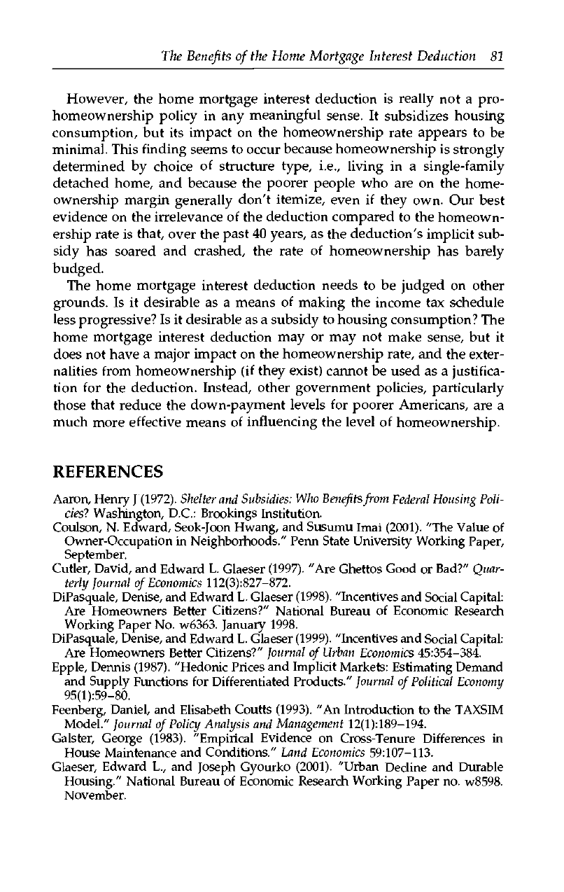
The Benefits of the Home Mortgage Interest Deduction 81

However, the home mortgage interest deduction is really not a pro-

homeownership policy in any meaningful sense. It subsidizes housing

consumption, but its impact on the homeownership rate appears to be

minimal. This finding seems to occur because homeownership is strongly

determined by choice of structure type, i.e., living in a single-family

detached home, and because the poorer people who are on the home-

ownership margin generally don't itemize, even if they own. Our best

evidence on the irrelevance of the deduction compared to the homeown-

ership rate is that, over the past 40 years, as the deduction's implicit sub-

sidy has soared and crashed, the rate of homeownership has barely

budged.

The home mortgage interest deduction needs to be judged on other

grounds. Is it desirable as a means of making the income tax schedule

less progressive? Is it desirable as a subsidy to housing consumption? The

home mortgage interest deduction may or may not make sense, but it

does not have a major impact on the homeownership rate, and the exter-

nalities from homeownership (if they exist) cannot be used as a justifica-

tion for the deduction. Instead, other government policies, particularly

those that reduce the down-payment levels for poorer Americans, are a

much more effective means of influencing the level of homeownership.

REFERENCES

Aaron, Henry J (1972). Shelter and Subsidies: Who Benefits from Federal Housing Poli-

cies?

Washington, D.C.: Brookings Institution.

Coulson, N. Edward, Seok-Joon Hwang, and Susumu Imai (2001). "The Value of

Owner-Occupation in Neighborhoods." Perm State University Working Paper,

September.

Cutler, David, and Edward L. Glaeser (1997). "Are Ghettos Good or Bad?" Quar-

terly Journal of Economics 112(3):827-872.

DiPasquale, Denise, and Edward L. Glaeser (1998). "Incentives and Social Capital:

Are Homeowners Better Citizens?" National Bureau of Economic Research

Working Paper No. w6363. January 1998.

DiPasquale, Denise, and Edward L. Glaeser (1999). "Incentives and Social Capital:

Are Homeowners Better Citizens?"

Journal

Urban Economics

45:354-384.

Epple, Dennis (1987). "Hedonic Prices and Implicit Markets: Estimating Demand

and Supply Functions for Differentiated Products."

Journal

Political Economy

95(l):59-80.

Feenberg, Daniel, and Elisabeth Coutts (1993). "An Introduction to the TAXSIM

Model." Journal of Policy Analysis and Management 12(1):189-194.

Galster, George (1983). "Empirical Evidence on Cross-Tenure Differences in

House Maintenance and Conditions." Land

Economics

59:107-113.

Glaeser, Edward L., and loseph Gyourko (2001). "Urban Decline and Durable

Housing." National Bureau of Economic Research Working Paper no. w8598.

November.

82 Glaeser & Shapiro

Glaeser, Edward L., and Joseph Gyourko (2002). "The Impact of Zoning on Hous-

ing Affordability." National Bureau of Economic Research Working Paper no.

w8835.

March.

Glaeser, Edward L., Jose A. Scheinkman, and Andrei Shleifer (1995). "Economic

Growth in a Cross-Section of Cities."

Journal

Monetary Economics

36(1):117-143.

Glaeser, Edward L, and Jesse M. Shapiro (2003). "Urban Growth in the 1990: Is

City Living Back?"

Journal

Regional Science

43(1):139-165, forthcoming.

Goodman, John L, Jr., and John B. Ittner (1992). "The accuracy of Homeowners'

Estimates of House Value."

Journal

Housing Economics

2(4):339-357.

Gordon, Roger H., James R. Hines, Jr., and Lawrence H. Summers (1987). "Notes

on the Tax Treatment of Structures." In The

Effects

Taxation

Capital

Accumu-

lation, Martin Feldstein (ed.). Chicago,

111.:

University of Chicago Press.

Green, Richard, and Michelle White (1997). "Measuring the Benefits of Homeown-

ing: Effects on Children."

Journal

Urban Economics

41(3):441-461.

Henderson, J. Vernon, and Yannis Ioannides (1983). "A Model of Housing Tenure

Choice."

American Economic

Review 73:98-113.

Kanemoto, Yoshitsugu (1990). "Contract Types in the Property Market."

Regional

Science

and

Urban Economics

20(l):5-22.

Katz, Lawrence F., Jeffrey R. Kling, and Jeffrey B. Liebman (2001). "Moving to

Opportunity in Boston: Early Results of a Randomized Mobility Experiment."

Quarterly Journal

Economics

116(2):607-654.

Mills,

Edwin S (1987). "Dividing up the Investment Pie: Have We Overinvested

in Housing?"

Federal Reserve

Bank of

Philadelphia

Business Review. March 1987

pp.

13-23.

Monroe, Albert (2001). "The Effects of Homeownership on Communities." Har-

vard University Dissertation. May 2001.

Oswald, Andrew J (1999). "The Housing Market and Europe's Unemployment:

A Non-Technical Paper." University of Warwick Working Paper.

Poterba, James (1984). "Tax Subsidies to Owner-Occupied Housing: An Asset-

Market Approach."

Quarterly Journal

Economics

99(4):729-752.

Poterba, James (1992). "Taxation and Housing: Old Questions, New Answers."

American

Economic

Review 82:237-242.

Rosen, Harvey S. (1979). "Housing Decisions and the U.S. Income Tax: An Econo-

metric Analysis."

Journal

Public Economics

ll(l):l-23.

Rosen, Harvey S. (1985). "Housing Behavior and the Experimental Housing Al-

lowance Program: What Have We Learned?" National Bureau of Economic Re-

search Working Paper no. wO657. May 1985.

Rosen, Harvey S., and Kenneth T. Rosen (1980). "Federal Taxes and Home Owner-

ship:

Evidence from Time Series."

Journal

Political Economy

88(l):59-75.

Rossi, Peter, and Eleanor Weber (1996). "The Social Benefits of Homeownership:

Empirical Evidence from the National Surveys." Housing

Policy Debate

7:37-81.

Shilling, James, C. F. Sirmans, and Jonathan Dombrow (1991). "Measuring Depre-

ciation in Single-Family Rental and Owner-Occupied Housing."

Journal

Hous-

ing

Economics

1:368-383.

Stein, Jeremy C. (1995). "Prices and Trading Volume in the Housing Market: A Model

with Down-Payment Effects."

Quarterly Journal

Economics

110(2):379-406.

Voith, Richard (1999). "Does the Federal Tax Treatment of Housing Affect the

Pattern of Metropolitan Development?"

Federal Reserve Bank

Philadelphia

Busi-

ness Review 3-16.