Guide for Environmentally Sustainable Investment Analysis Based on ASTM E3200

NIST Advanced Manufacturing Series 200-11

Guide for Environmentally Sustainable

Investment Analysis Based on ASTM E3200

A method for investment analysis that incorporates environmental

impact with a focus on manufacturing

Douglas Thomas

Anand Kandaswamy

David Butry

This publication is available free of charge from:

https://doi.org/10.6028/NIST.AMS.200-11

NIST Advanced Manufacturing Series 200-11

Guide for Environmentally Sustainable

Investment Analysis Based on ASTM E3200

Douglas Thomas

Anand Kandaswamy

David Butry

Applied Economics Office

Engineering Laboratory

This publication is available free of charge from:

https://doi.org/10.6028/NIST.AMS.200-11

March 2021

U.S. Department of Commerce

Gina M. Raimondo, Secretary

National Institute of Standards and Technology

James K. Olthoff, Performing the Non-Exclusive Functions and Duties of the Under Secretary of Commerce

for Standards and Technology & Director, National Institute of Standards and Technology

Certain commercial entities, equipment, or materials may be identified in this

document in order to describe a n experimental procedure or concept adequately.

Such identification is not intended to imply recommendation or endorsement by the

National Institute of Standards and Technology, nor is it intended to imply that the

entities, materials, or equipment are necessarily the best available for the purpose.

National Institute of Standards and Technology Advanced Manufacturing Series 200-11

Natl. Inst. Stand. Technol. Adv. Man. Ser. 200-11, 47

pages (March 2021)

This publication is available free of charge from:

https://doi.org/10.6028/NIST.AMS.200-11

This publication is available free of charge from: https://doi.org/10.6028/NIST.AMS.200-11 .

Abstract

This guide presents techniques for evaluating manufacturing investments from the

perspective of environmentally sustainable manufacturing by pairing economic methods of

investment analysis with environmental aspect of manufacturing, including manufacturing

processes. The methods are based on ASTM E3200 and, although the focus is on

manufacturing, they can be applied under other circumstances (e.g., construction industry

investments, agriculture, or mining). The economic techniques include net present value,

internal rate of return, payback period, and hurdle rate. The guide also includes sensitivity

analyses with a focus on Monte Carlo techniques. The methods presented can be used by

manufacturers, regardless of size or complexity, to make environmentally sustainable

decisions, including but not limited to whether to embark on an investment, discontinue a

manufacturing line, and invest or re-invest in a new project or factory.

Key words

Investment analysis; manufacturing; environmental sustainability

This publication is available free of charge from: https://doi.org/10.6028/NIST.AMS.200-11 .

Table of Contents

1. Introduction...................................................................................................................... 1

2. Sustainable Investment Analysis .................................................................................... 3

Step 1.1 - Initial Assessment: Identify Economic Method and ApplyError! Bookmark not

defined.

Step 1.2 - Initial Assessment: Conduct Environmental Assessment.. Error! Bookmark not

defined.

Step 2 - Consolidate Assessments: Evaluate whether there is a Tradeoff ............................ 6

Step 3 - Evaluate Tradeoff .................................................................................................. 12

Step 4 - Sensitivity Analysis ............................................................................................... 15

Step 5 – Rank the Investments ............................................................................................ 17

References .............................................................................................................................. 18

Appendix A: Economic Methods ......................................................................................... 20

Appendix B: Examples ......................................................................................................... 29

List of Tables

Guide

Table 2.1: Examples of Decision Types ............................................................................ 5

Table 2.2: Appropriate Application of Financial Economic Methods .............................. 5

Table 2.3: Consolidating Assessments: Combinations of Outcomes .... Error! Bookmark

not defined.

Table 2.4: Sensitivity Analysis Example ......................................................................... 17

Appendix A

Table A-1: Example Cash Inflows and Outflows by Year for NPV Calculations .......... 21

Table A-2: IRR Decision Matrix ..................................................................................... 24

Table A-3: Example Cash Inflows and Outflows by Year for NPV Calculations ......... 24

Appendix B

Table B-1: Annual Cash Flows for Example 2................................................................ 30

Table B-2: Annual Cash Flows for Example 5................................................................ 34

Table B-3: Annual Cash Flows for Example 6................................................................ 35

Table B-4: Annual Cash Flows for Example 8................................................................ 37

Table B-5: Environmental and Economic Assessment ................................................... 40

Table B-6: Pairwise Comparisons ................................................................................... 40

Table B-7: Pairwise Comparison ..................................................................................... 41

List of Figures

Guide

Figure 2.1: Five Steps for Environmentally Sustainable Investment Analysis ................. 4

Figure 2.2: Decision Tree for Accept/Reject Decisions .................................................... 8

iii

This publication is available free of charge from: https://doi.org/10.6028/NIST.AMS.200-11 .

Figure 2.3: Decision Tree where Environmental Analysis is Accept/Reject Decision and

Economic Analysis is Priority/Ranking Decision ............................................................. 9

Figure 2.4: Decision Tree where Economic Analysis is Accept/Reject Decision and

Environmental Analysis is Priority/Ranking Decision ...................................................... 9

Figure 2.5: Decision Tree for Design, Size, and Ranking/Priority Decisions, One

Alternative ....................................................................................................................... 10

Figure 2.6: Decision Tree for Design, Size, and Ranking/Priority Decisions, Multiple

Alternatives ...................................................................................................................... 11

Figure 2.7: Illustration of Pairwise Comparison.............................................................. 12

Appendix A

Figure A-1: Example of Net Cash Flows by Year......................................................... 22

Appendix B

Figure B-1: Decision Tree for Example 3 ....................................................................... 32

Figure B-2: Decision Tree for Example 4 ....................................................................... 33

Figure B-3: Decision Tree for Example 5 ....................................................................... 34

Figure B-4: Decision Tree for Example 7 ....................................................................... 37

Figure B-5: Decision Tree for Example 9 ....................................................................... 39

This publication is available free of charge from: https://doi.org/10.6028/NIST.AMS.200-11 .

1. Introduction

This guide presents techniques for evaluating manufacturing investments from the

perspective of environmentally sustainable manufacturing by pairing economic methods

of investment analysis with environmental aspect of manufacturing, including

manufacturing processes. Although the focus is on manufacturing, the methods can be

applied under other circumstances (e.g., construction industry investments, agriculture, or

mining). The methods presented are based on ASTM E3200.

The economic techniques discussed include net present value, internal rate of return,

payback period, and hurdle rate. These four techniques are deterministic, meaning that

they deal with known values that are certain. Probabilistic considerations play no role in

determining how these four techniques are deployed. The guide will also move beyond

standard deterministic techniques to look at probabilistic methods like the concept of

sensitivity analyses, with a focus on Monte Carlo analyses.

The techniques can be used by manufacturers, regardless of size or complexity, to make

environmentally sustainable decisions, including but not limited to whether to embark on

an investment, discontinue a manufacturing line, and invest or re-invest in a new project

or factory. To outline all possible decision types would constitute another guide.

This guide does not assume specific knowledge of financial techniques on the part of the

user, besides some knowledge of discounting. The interested reader is encouraged to

follow up and consult outside readings to cover financial techniques beyond the scope of

this guide. The guide also uses US dollars, percent change in environmental aspects of

manufacturing, and unit change in environmental aspects of manufacturing as its primary

units.

Techniques for evaluating manufacturing investments from the perspective of

environmentally sustainable manufacturing are presented in this guide. It pairs economic

methods of investment analysis with environmental aspects of manufacturing. The

method presented includes five steps:

1. Initial assessment

2. Consolidate assessments

3. Evaluate tradeoff

4. Sensitivity analysis

5. Rank the investments

There are four types of investment decisions for which four methods of financial

economic analysis are applied along with metrics (indicators) for environmental aspects

of manufacturing. Methods apply to specific decision types. When combined, financial

economic analysis and metrics for environmental aspects of manufacturing result in a

combination of financial and environmental outcomes, each associated with an additional

procedure.

This publication is available free of charge from: https://doi.org/10.6028/NIST.AMS.200-11 .

This guide provides a method for evaluating investments in terms of their financial merits

and environmental merits. This guide can be used to answer whether an investment is

both economical and environmentally sustainable or if there is a tradeoff between the

environmental aspects of manufacturing and profitability. A tradeoff means there is not a

clear best solution and user discretion is required. If there are tradeoffs, this guide

provides methods for framing those tradeoff decisions.

The financial merits for this guide are, typically, from the individual stakeholder

perspective (e.g., owners and/or investors) or from the perspective of a selection of

stakeholders. It is up to the user to decide what financial changes are relevant to them.

For instance, if there is a financial cost borne by a third party, the user may opt to exclude

it from their analysis, as it is not relevant for them. The environmental merits are from a

multi-stakeholder perspective (e.g., societal level) and should follow established

standards for evaluating environmental aspects of manufacturing. That is, environmental

aspects of manufacturing should not be excluded simply because they do not affect the

user.

This publication is available free of charge from: https://doi.org/10.6028/NIST.AMS.200-11 .

2. Sustainable Investment Analysis

As seen in Figure 2.1, the method presented includes an iterative process incorporated

into a five-step procedure. The first step requires an economic and environmental

assessment. The economic assessment evaluates the financial merits of an investment

while the environmental assessment evaluates the environmental aspects of

manufacturing resulting from the investment. Both assessments evaluate potential

investments relative to the status quo (i.e., base case).

Step 2 (Consolidate Assessments) and Step 3 (Evaluate Tradeoff) bring these assessments

together for comparison and consider any tradeoffs. The outcome of the economic and

environmental assessment results in any one of several outcome combinations (e.g., a

financially economical investment that is not environmentally favorable), each having its

own implications. Depending on the outcomes, the first three steps may need to be

repeated. Step 4 (Sensitivity Analysis) evaluates the impact of uncertainty in the data.

There are often variables that are not known with certainty and there is a need to consider

the possibility of having different values, resulting in different outcomes. The final step,

Step 5, is to rank the investments. A few terms are used in discussing the method,

including the following:

• Evaluation: The execution of the complete method discussed in this guide,

including Steps 1 through 5 and the repeating of any steps, that results in ranking

the status quo and potential investments.

• Iteration: An instance of applying steps 1 through 3

• Comparison or Pairwise Comparison: Where an investment is compared to one

other investment using steps 1 through 3.

• Assessment: Applying either economic or environmental methods to determine

whether each investment is financially economical, environmentally favorable,

accepted, or rejected depending on the decision type.

Multiple economic and environmental assessments are completed and compared. The

relation of each economic/environmental assessment is based on the change that results

from a particular investment from a comparison case. For an economic assessment, it is

the change in finances that result in the investment. For an environmental assessment, it

is the change in the environmental aspects of manufacturing that results from the

investment.

Step 1.1 - Initial Assessment: Identify Economic Method and Apply

The first part of Step 1 (i.e., Step 1.1) is an economic analysis. There are four types of

economic decisions: accept/reject, design, size, and priority/ranking. An accept/reject

decision does not compare investments, but rather determines whether an investment

meets a threshold level of performance. A design decision pertains to choices between

variations of an investment where only one can be selected. A sizing decision is one that

involves different magnitudes within an investment, where only one magnitude can be

This publication is available free of charge from: https://doi.org/10.6028/NIST.AMS.200-11 .

Figure 2.1: Five Steps for Environmentally Sustainable Investment Analysis

selected. A ranking decision includes prioritizing and then selecting one or more

investments from a group when a budget is not enough to fund all cost-effective

investments. Examples for each of the decision types are presented in Table 2.1.

Four basic approaches for financial economic analysis are discussed in this guide: net

present value, internal rate of return, hurdle rate, and payback period. Different

approaches are appropriate for each of the four decision types, as defined in Table 2.2.

Net present value is appropriate for three of the decision types: accept/reject, design, and

size. Internal rate of return is appropriate for all four decision types, while hurdle rate and

payback period are only appropriate for accept/reject decisions. Appendix A details each

of the methods for financial economic analysis.

Step 1.2 - Initial Assessment: Conduct Environmental Assessment

Step 1.2 is to examine the environmental aspects of manufacturing of the proposed

investments. This guide is not intended to contradict or circumvent the provisions of ISO

14025, ISO 14040, ISO 14044, ISO 14067, ISO14049, or ISO 21930 and encourages

their use, and, if the assessment is of a building, ASTM E2921. For the purpose of the

method presented here, the user can either use a percent change in environmental aspects

of manufacturing or a unit change (e.g., tons of carbon dioxide emitted). These

environmental impacts could be measured using methods presented in E3096.

Step 5

Rank

Investments

Step 4

Sensitivity

Analysis

(Optional)

Step 3

Evaluate

Tradeoff

Step 2

Consolidate

Assessments

Step 1

Initial

Assessment

Conduct

environmental

assessment

Evaluate whether

there is a

tradeoff

No tradeoff:

evaluate

investment

Tradeoff: identify

tradeoff metric

and apply

Select sensitivity

analysis and

apply

Reject

Identify

economic

method and

apply

This publication is available free of charge from: https://doi.org/10.6028/NIST.AMS.200-11 .

Table 2.1: Examples of Decision Types

Accept/Reject

Is an additive manufacturing system cost effective?

Is a new climate control system cost effective?

Is a new robotic system cost effective?

Design

What robotic system is the most cost effective?

What HVAC control system is the most cost effective?

Which milling machine is the most cost effective?

Is it more cost effective to use steel or aluminum materials?

Size

How many machine tools should be replaced?

What size of lathe is most cost effective?

Priority or Ranking

Is it more cost effective to invest in new machine tools or a

new HVAC control system?

We have five proposed investments but can only afford a

selection of them. Which investments do we choose?

Table 2.2: Appropriate Application of Financial Economic Methods

Net Present Value

Internal Rate of Return

Hurdle Rate

Payback Period and Discounted

Payback Period

Accept/Reject

Design

Size

Priority or Ranking

1: Note significant limitations

2: Appropriate when incremental discounted costs and benefits are

considered (i.e., the difference in costs/benefits between two

investments). To decide between more than two options, pairwise

comparisons are necessary.

ASTM E3096: Standard Guide for Definition, Selection, and Organization of Key

Performance Indicators for Environmental Aspects of Manufacturing provides a

procedure for identifying key performance indicators for the environmental aspects of

manufacturing processes. It also provides a procedure for normalizing key indicators,

assigning weights, and aligning them with environmental objectives.

One additional standard that can be utilized for evaluating the environmental aspects of

manufacturing is ASTM E2986. This guide provides guidance to develop procedures for

evaluating environmental sustainability performance of processes in manufacturing. This

This publication is available free of charge from: https://doi.org/10.6028/NIST.AMS.200-11 .

guide addresses a number of issues, including setting boundaries and identifying process

and equipment related parameters.

The methods presented here in this guide are designed to make comparisons across a

single metric (indicator) of environmental aspects of manufacturing measured as either

it’s percent change or the unit change resulting from the investment. For simplicity, the

guide relies on percent change. To use unit change, the user can simply replace the

measure of percent change with the preferred units. ASTM E3096 provides methods of

defining and selecting key performance indicators, including a process for aggregating

multiple indicators into a single metric.

For this guide, an investment is considered environmentally favorable if the percent

change or unit change is less than or equal to zero (i.e., does not increase the

environmental impact). It is environmentally unfavorable if the percent change or unit

change is greater than zero (i.e., an increase in environmental impact). In the case where

Step 1 and Step 2 are being repeated (discussed below), the denominator, environmental

impact of the status quo or 



 in the equation below, does not change. Moreover, in the

first iteration 



 equals 



; however, in subsequent iterations they will not be

equivalent. This is done so that one percentage point of environmental impact always

equals the same nominal amount throughout the evaluation. The percent change between

two investment options  and  can then be estimated:

Equation 1























′

 100

where





= Percent change in environmental impact between option a (i.e., base case) and

potential investment option b





′ = Environmental impact of the status quo (i.e., initial base case), which does not

change throughout the evaluation





= Environmental impact of investment option 





= Environmental impact of investment option 

Step 2 - Consolidate Assessments: Evaluate whether there is a Tradeoff

As presented in the first four columns of Table 2.3, bringing the environmental

assessment together with the economic assessment results in a series of potential outcome

combinations, referred to as scenarios, for each investment being assessed. Therefore,

one might be comparing investments from multiple scenarios (or the same scenario)

within a decision type. In the following sections each decision type is discussed with

references made to the scenarios in Table 2.3, along with a decision tree for each decision

type. The scenarios in the decision trees correspond with those in Table 2.3.

This publication is available free of charge from: https://doi.org/10.6028/NIST.AMS.200-11 .

Accept/Reject Decisions: If a decision is an accept/reject decision for both the

environmental and financial assessment (i.e., Scenarios 1.1 through 1.4), then the

investment is only acceptable if both assessments are accepted (see Scenario 1.1) and,

therefore, no scenarios are compared. This process can be traced in the decision tree in

Figure 2.2.

Accept/Reject with Priority/Ranking Decision: If a decision is a combination of

accept/reject and ranking/priority (i.e., Scenarios 2.1 through 3.4), then all but two of the

scenarios are rejected, as seen in the decision trees in Figure 2.3 and Figure 2.4. There

could be multiple investments categorized as Scenario 2.1 or 3.1. If this is the case, then

there is a comparison based on either the financial assessment (applicable to Scenario

2.1) or the environmental assessment (applicable to Scenario 3.1).

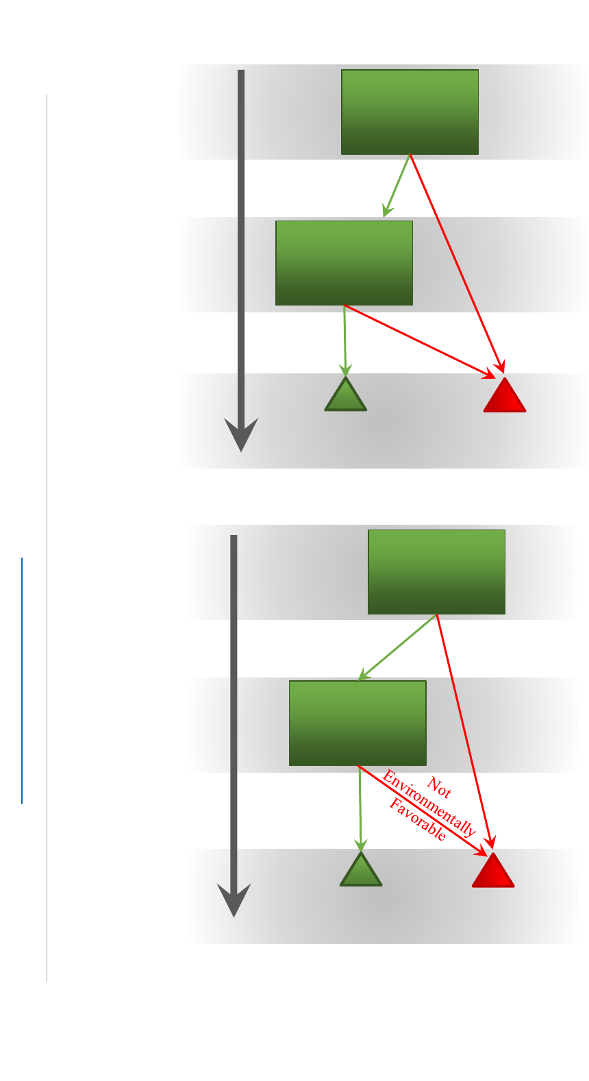
Design, Size, and Ranking/Priority Decisions: If a decision is a design, size, or

ranking/priority decision type (i.e., Scenarios 4.1 through 4.4), then there are four

possible scenarios for each investment being evaluated. A series of guidelines need to be

followed for this decision type. Scenarios where only one alternative to the status quo is

considered (see Figure 2.5) are examined separately from those that have two or more

alternatives (see Figure 2.6).

One Alternative: As seen in Figure 2.5, there are three potential outcomes for those

instances where there is only one alternative to the status quo. The first potential outcome

is when the alternative is ranked better than the status quo in both environmental terms

and economic terms (see Scenarios 4.1). In this case, the alternative is preferred to the

status quo. The second potential outcome is that the alternative is ranked worse in both

Table 2.3: Consolidating Assessments: Combinations of Outcomes

Decision Type

Scenario

Environmental Assessment

Economic/Financial Assessment

Action

Accept/Reject

1.1

Acceptable Investment

1.2

Reject

1.3

Reject

1.4

Reject

Environ:

Accept/Reject -

Economic:

Ranking/Priority

2.1

Financially Economical

Select on $

2.2

Not Financially Economical

Reject

2.3

Reject

Financially Economical

Reject

2.4

Reject

Not Financially Economical

Reject

Environ:

Ranking/Priority

- Economic:

Accept/Reject

3.1

Environmentally Favorable

Select on Env.

3.2

Not Environmentally Favorable

Reject

3.3

Environmentally Favorable

Reject

3.4

Not Environmentally Favorable

Reject

Design, Size,

Ranking/Priority

4.1

Environmentally Favorable

Financially Economical

Pairwise Comparison

4.2

Not Environmentally Favorable

Not Financially Economical

Reject

4.3

Not Environmentally Favorable

Financially Economical

Consider Tradeoff/

Pairwise Comparison

4.4

Environmentally Favorable

Not Financially Economical

Consider Tradeoff/

Pairwise Comparison

This publication is available free of charge from: https://doi.org/10.6028/NIST.AMS.200-11 .

Figure 2.2: Decision Tree for Accept/Reject Decisions

economic and environmental terms (see Scenario 4.2). In this case, the status quo is

preferred to the alternative being considered.

The last potential outcome has a tradeoff when compared to the status quo (see Scenarios

4.3 and 4.4). The tradeoff involves one of two situations: 1) an economical investment

that increases environmental impact or 2) an investment that is not economical that

decreases environmental impact. In this case the user must decide whether the investment

with the tradeoff is better or worse than the status quo. A selection of tradeoff metrics is

discussed in Step 3 shown in Section 6.6.

Two or more alternatives: For instances where there is more than one alternative to the

status quo, the user follows the decision tree in Figure 2.6. Similar to Figure 2.5, if an

investment is not economical and it is not environmentally favorable (Scenario 4.2), then

that investment is not preferred to the status quo. Investments that are both economical

and environmentally favorable must be compared in a pairwise comparison, as discussed

below. If there is a tradeoff (Scenarios 4.3 and 4.4), then the user must determine if the

tradeoff is preferred to the status quo. A selection of tradeoff metrics is discussed in

Environmental

Analysis

(Accept/Reject)

Economic

Analysis

(Accept/Reject)

Reject

(Scenario 1.2-1.4)

(Scenario 1.1)

Reject

This publication is available free of charge from: https://doi.org/10.6028/NIST.AMS.200-11 .

Figure 2.3: Decision Tree where Environmental Analysis is Accept/Reject Decision and

Economic Analysis is Priority/Ranking Decision

Figure 2.4: Decision Tree where Economic Analysis is Accept/Reject Decision and

Environmental Analysis is Priority/Ranking Decision

Economic

Analysis

(Ranking)

Environmental

Analysis

(Accept/Reject)

Reject

(Scenario 2.2-2.4)

Select on $

(Scenario 2.1)

Financially

Economical

Not Financially

Economical

Reject

Economic

Analysis

(Accept/Reject)

Environmental

Analysis

(Ranking)

Reject

(Scenario 3.2-3.4)

Select on Env.

(Scenario 3.1)

Reject

Environmentally

Favorable

This publication is available free of charge from: https://doi.org/10.6028/NIST.AMS.200-11 .

Step 3 shown in Section 6.5. If the tradeoff is preferred, then a pairwise comparison must

be made between the other alternatives.

Pairwise Comparison: In the case where there are multiple alternative investments, it

may be necessary to conduct a pairwise comparison where each investment is compared

relative to each of the other investments. The result will rank all the investments. This

requires repeating Step 1 and Step 2, but only considering two investments at a time. In

each comparison, one investment is selected as the new status quo (i.e., a new base case)

while the other investment is treated as a potential alternative investment to the new

status quo. Each of the comparisons will result in using Figure 2.5 to determine if the

alternative is preferred to the new status quo. Additional investments then can be

compared to determine where they rank relative to the others.

Figure 2.5: Decision Tree for Design, Size, and Ranking/Priority Decisions, One

Alternative

* These two boxes represent the same environmental analysis a nd not two separate or different analyses.

Economic

Analysis

(Ranking)

Environmental

Analysis

(Ranking)*

Environmental

Analysis

(Ranking)*

Reject: Status Quo (i.e., base

case) Outranks the Alternative

(Scenario 4.2, 4.3, 4.4)

Accept: Alternative Outranks the

Status Quo (i.e., base case)

(Scenario 4.1, 4.3, 4.4)

Environmentally

Favorable

Not Environmentally

Favorable

Financially

Economical

Not Financially

Economical

Evaluate Tradeoff

(Scenario 4.3, 4.4)

Favorable

Not Favorable

This publication is available free of charge from: https://doi.org/10.6028/NIST.AMS.200-11 .

Figure 2.7 illustrates how investments are compared in a pairwise comparison. In this

example, it was determined that investments A, B, and C were each preferred over the

status quo. A second iteration compared investment A with investment B, which resulted

in determining that A is preferred to B. A second iteration is needed to determine if

investment C is preferred to A and/or B, putting it before, between, or after A and B in

Figure 2.7. Investment C can be compared to investment A to determine if it is ranked 1

If investment C is not preferred to A, then it must be compared to investment B to

determine whether it is ranked 2

or 3

. Note that in the case where Step 1 and Step 2

are being repeated, the denominator 



 from the equation from Step 1.2 does not

change when using a percent change, as previously discussed.

Figure 2.6: Decision Tree for Design, Size, and Ranking/Priority Decisions, Multiple

Alternatives

* These two boxes represent the same environmental analysis a nd not two separate or different analyses.

Economic

Analysis

(Ranking)

Environmental

Analysis

(Ranking)*

Environmental

Analysis

(Ranking)*

Reject: Status Quo (i.e., base

case) Outranks the Alternative

(Scenario 4.2, 4.3, 4.4)

Environmentally

Favorable

Not Environmentally

Favorable

Financially

Economical

Not Financially

Economical

Evaluate Tradeoff

(Scenario 4.3, 4.4)

Not Favorable

Favorable

Pairwise Comparison

(Scenario 4.1, 4.3, 4.4)

This publication is available free of charge from: https://doi.org/10.6028/NIST.AMS.200-11 .

Figure 2.7: Illustration of Pairwise Comparison

Moreover, in the first iteration 



 equals 



; however, in subsequent iterations they

will not be equivalent. This is done so that one percentage point of environmental impact

always equals the same nominal amount of environmental impact throughout the

evaluation.

Step 3 - Evaluate Tradeoff

A tradeoff exists when: 1) a scenario includes an investment that is not environmentally

favorable but is financially economical or 2) a scenario includes an investment that is not

financially economical but is environmentally favorable. Each of these has a set of

metrics for evaluation.

Not Environmentally Favorable but Financially Economical: There are four metrics

that are useful for considering a tradeoff where the investment is not environmentally

favorable: maximum impact, the net present value per percent change in environmental

impact (NPVP), environmental hurdle rate, and the net present value elasticity (NPVE).

Each of these are discussed below.

Not Financially Economical but Environmentally Favorable: There are four metrics

that are useful for considering a tradeoff where the investment is not financially

economical, but is environmentally favorable: maximum environmental expenditure,

maximum environmental expenditure rate (MEER), net present value per percent change

in environmental impact (NPVP), and the net present value elasticity (NPVE). Each of

these metrics are discussed below.

Maximum Impact: The maximum impact is the largest acceptable increase in

environmental impact. It can either be in percent change in impact or in units (e.g., tons

of CO2). It is compared to the change in impact for the investment being evaluated and is

applicable when the change in environmental impact is positive (i.e., an increase in the

impact). If the impact of the investment is greater than the maximum impact, then the

investment is rejected or ranked lower when compared to the status quo. For instance, if

Investment A

Investment B

2nd

1st

Investment C

Status Quo

Last

Rank

This publication is available free of charge from: https://doi.org/10.6028/NIST.AMS.200-11 .

an investment increases the environmental impact by 10 % and the maximum impact for

the investor is 5 %, then the investment would be ranked lower than the status quo.

Net Present Value per Percent Change in Environmental Impact (NPVP): This value

is the average increase or decrease in income brought about by each percentage point

change (or unit change) in environmental impact. It is calculated as:

Equation 2









where

 = Net Present Value per Percent Increase in Environmental Impact

 = Net Present Value (see Appendix A1.1)





= Percent change in environmental impact between option a (i.e., base case) and

potential investment option b (see Equation 1)

This calculation is only used when there is a tradeoff between cost effectiveness and

environmental impact, which occurs when both NPV and 



are both positive

(financially economical but not environmental favorable) or both negative (not financial

economical but environmental favorable). In the former situation, higher values are

better, as this represents income or cost savings. In the latter situation, lower values are

better, as this represents expenditures. Values should not be compared between these two

categories, as one represents an expenditure while the other represents income or cost

savings.

Environmental Hurdle Rate: The environmental hurdle rate is a value selected by the

decision maker and represents the net present value of income or cost savings needed to

compel a one percent increase (or one-unit increase) in environmental impact. It is

applicable in the case where an investment is financially economical but not

environmentally favorable. If the investment’s NPVP exceeds the decision maker’s

environmental hurdle rate, then the investment is considered acceptable or ranked higher

when compared to the status quo.

To illustrate the environmental hurdle rate, consider an investment with an NPVP of

$4500 per percent (or unit) increase in environmental impact. If the decision maker has a

$10 000 environmental hurdle rate, that is, they are willing to increase their

environmental impact by 1 % in return for a $10 000 increase; then, this investment is not

preferred.

This publication is available free of charge from: https://doi.org/10.6028/NIST.AMS.200-11 .

Maximum Environmental Expenditure: The maximum environmental expenditure is

the total amount the user is willing to pay to reduce environmental impact after all other

financial benefits are considered. This metric is intended to be used when the net present

value is negative. The maximum expenditure is compared to the absolute value of net

present value. If the maximum value is greater than the net present value, then the loss is

bigger than the willingness to pay and the alternative is rejected or ranked lower when

compared to the status quo. For instance, if an investment has a net present value of

$-25 000 and the investor has a maximum environmental expenditure of $30 000, then

the investment would be ranked higher than the status quo.

Maximum Environmental Expenditure Rate (MEER): The MEER is a value selected

by the decision maker to represent the maximum they are willing to pay to decrease the

environmental impact by one percent (or one unit). It is applicable in the case where an

investment is not financially economical but is environmentally favorable. If the NPVP is

below the MEER, then this investment is considered acceptable or ranked higher when

compared to the status quo. For instance, if the NPVP is $5000 and the MEER for the

investor is $2500 per percentage point decrease, then the investment would be ranked

below the status quo.

Net Present Value Elasticity (NPVE): The net present value elasticity is the percent

increase in net present value per one percent increase in environmental impact. It is

calculated as:

Equation 3



















 





where





= Net present value for the status quo





= Net present value for investment b





= Percent change in environmental impact between option a (i.e., base case) and

potential investment option b (see Equation 1)

This value informs decision makers on the relative tradeoff between the environment and

income/cost. For investments that are financially economical but not environmentally

favorable, a higher NPVE is considered better. For investments that are environmentally

favorable but not financially economical, a lower NPVE is better. The NPVE can be

compared between investments, but the NPVE for investments that are financially

economical but not environmentally favorable should not be compared with the NPVE

for investments that are environmentally favorable but not financially economical.

This publication is available free of charge from: https://doi.org/10.6028/NIST.AMS.200-11 .

Step 4 - Sensitivity Analysis

The techniques discussed in the previous section of the guide are what are known as

deterministic techniques, meaning that there are single values assumed for calculations

incorporated into the analysis. Deterministic techniques assume the manufacturer knows

with complete certainty all the variables in the relevant equation, whether they are future

payment streams or interest/discount rates. Every part of every equation is assumed to be

known with absolute confidence.

In most situations that a manufacturer faces, at least some of the values needed to make a

decision are not completely transparent or may be known with only partial certainty.

To account for this uncertainty, the manufacturer can turn to probabilistic techniques

such as a sensitivity analysis. Sensitivity analysis quantifies the change in results due to

variation in one or more input values.

For example, suppose the manufacturer is deciding whether to invest in some capital

machinery, and will base the decision on the NPV. Assume that a manufacturer faces

uncertainty about the opportunity cost of capital, which affects the discount rate for an

investment. The choice of discount rate may determine that investment decision. To

account for the uncertainty, the manufacturer can use the concept of a risk-adjusted

discount rate (RADR). By assigning probabilities to each of a range of discount factors,

the manufacturer can perform a more sophisticated analysis than by simply choosing a

discount rate deterministically. Suppose that the manufacturer allows for r, the discount

rate, to take a range of values. Assume r could be 5 %, 6 %, or 7 %. Further, assume the

probability of each of these three values is equal, at one-third probability each. By

calculating each of the r’s and assigning a one-third probability to them, the manufacturer

will have a better understanding of the range of possibilities of investing in the capital

machinery.

A more specific type of sensitivity analysis, and one that is commonly deployed when

dealing with probabilistic decision-making is the Monte Carlo analysis. The Monte Carlo

method uses repeated random sampling to generate simulated data to use with a

mathematical model. Monte Carlo analysis can be performed using a variety of computer

software packages.

Monte Carlo analysis operates in the following manner: Each variable in the model is

assigned a likely range of outcomes, based on prior data analysis. Each time the model is

run, the computer program will randomly assign values to those variables based on user

specified distributions and ranges. The model is typically run for thousands of iterations,

with new randomly generated input variables each time. The outcomes across these

iterations are tabulated and summarized into a probability distribution.

Rather than a deterministic base case scenario, a Monte Carlo simulation typically

produces a range of outcomes that can be used to develop a distribution.

This publication is available free of charge from: https://doi.org/10.6028/NIST.AMS.200-11 .

The caveat with Monte Carlo is that the results are shaped by the underlying assumptions.

As in any model, the accuracy of the assumptions is key. With a Monte Carlo simulation,

the ranges of possible values assigned to each variable constitute a critical set of

assumptions on which the whole undertaking rests, along with the methodology for

converting random numbers generated by the computer into values within these ranges.

The great benefit of the Monte Carlo analysis is that the values will be selected randomly

using the algorithm of the chosen software package. Because there is difficulty in

approximating randomness, a computer package can do a relatively accurate job of

approximating randomness (although it will be just an approximation since no computer

program can generate true randomness).

One of the challenges that arises in sensitivity/uncertainty analysis is that some

investments might end up being recategorized as a different scenario from Table 2.3. The

probabilistic nature of the analysis means that the underlying investments will be

categorized in different ways, depending on the state of the world generated by the

changing scenarios. Currently, there is no known software package that can be applied to

account for this issue; thus, one would have to develop their own coded model that makes

this calculation. The outcome would estimate the ranking of each investment for each

iteration.

Monte Carlo analysis is further discussed in Section 3.1 of NIST Advanced

Manufacturing Series 200-5.

NIST’s Monte Carlo tool can be used to implement this

type of analysis.

Sensitivity Analysis Example: Assume that a piece of capital machinery in a

manufacturer’s plant will wear out after some number of years. However, the

manufacturer does not know for sure when the machinery will wear out, but there is

reason to believe that the machinery could fail in any year from year 4 to year 8. Further,

suppose there is a probability of occurrence associated with each year of obsolescence,

which in this scenario is assumed to be known for each of the five years under

consideration. For this illustration, the replacement cost does not vary based on the year

of replacement and is always $100 000. A sensitivity factor (created exclusively for this

example) is then applied to each replacement cost by year. The sensitivity factor can be

generated through any number of software packages. This in turn provides the expected

present value of the cost for each year.

By applying sensitivity analysis, the manufacturer can evaluate the range of possible

replacement costs, based on the year when the capital machinery finally wears out and

can budget for those scenarios, thus reducing the risk to the firm. Looking at Table 2.4,

notice that in this instance the sum of the probabilities of a failure occurring in the second

column totals one. Furthermore, this example assumes that the replacement cost is

always the same, no matter what year it was incurred. The values generated in the fourth

column are artificial examples generated for the purposes of this example. What is

Thomas, Douglas. 2017. Investment Analysis Methods: A Practitioner’s Guide to Understanding the Basic Principles for Investment

Decisions in Manufacturing. NIST Advanced Manufacturing Series 200 -5. https://doi.org/10.6028/NIST.AMS.200-5

This publication is available free of charge from: https://doi.org/10.6028/NIST.AMS.200-11 .

important to note is that the product of the replacement cost and the sensitivity values of

present value savings generate the expected present value of cost.

Table 2.4: Sensitivity Analysis Example

Year for Capital

Machinery

Replacement

Probability

Occurrence

Replacement

Cost

Sensitivity of

Present Value

Savings (10 %

Discount

Rate)

Expected

Present

Value of

Cost

0.2

100 000

0.2

400

0.3

100 000

0.225

6750

0.1

100 000

0.456

4560

0.15

100 000

0.178

2670

0.25

100 000

0.676

16900

Step 5 – Rank the Investments

The last step of this process is to rank the investments based on the analysis. Investments

falling into Scenario 1.1 through 1.4 in Table 2.3 will either be accepted or rejected. For

the other decision categories, the user selects one or more investments based on the

ranking of the investments.

This publication is available free of charge from: https://doi.org/10.6028/NIST.AMS.200-11 .

References

ASTM. E1057: Standard Practice for Measuring Internal Rate of Return and Adjusted

Internal Rate of Return for Investments in Buildings and Building Systems. West

Conshohocken, PA.

ASTM. E1369: Standard Guide for Selecting Techniques for Treating Uncertainty and

Risk in the Economic Evaluation of Buildings and Building Systems. West

Conshohocken, PA.

ASTM. E2114: Standard Terminology for Sustainability Relative to the Performance of

Buildings. West Conshohocken, PA.

ASTM. E2921: Standard Practice for Minimum Criteria for Comparing Whole Building

Life Cycle Assessments for Use with Building Codes, Standards, and Rating Systems.

West Conshohocken, PA.

ASTM. E2986: Standard Guide for Evaluation of Environmental Aspects of

Sustainability of Manufacturing Processes. West Conshohocken, PA.

ASTM. E2987/E2987M: Standard Terminology for Sustainable Manufacturing. West

Conshohocken, PA.

ASTM. E3096: Standard Guide for Definition, Selection, and Organization of Key

Performance Indicators for Environmental Aspects of Manufacturing Processes. West

Conshohocken, PA.

ASTM. E3200: Standard Guide for Investment Analysis in Environmentally Sustainable

Manufacturing. West Conshohocken, PA.

ASTM. E833: Standard Terminology of Building Economics. West Conshohocken, PA.

International Organization for Standardization. ISO 14025: Environmental Labels and

Declarations – Type III Environmental Declarations – Principles and Procedures.

Geneva, Switzerland.

International Organization for Standardization. ISO 14040: Environmental Management

– Life Cycle Assessment – Principles and Framework. Geneva, Switzerland.

International Organization for Standardization. ISO 14044: Environmental management -

- Life cycle assessment -- Requirements and guidelines. Geneva, Switzerland.

International Organization for Standardization. ISO 14049: Environmental management -

- Life Cycle Assessment -- Illustrative Examples on How to Apply ISO 14044 to Goal

and Scope Definition and Inventory Analysis. Geneva, Switzerland.

International Organization for Standardization. ISO 14067: Greenhouse gases -- Carbon

Footprint of Products -- Requirements and Guidelines for Quantification and

Communication. Geneva, Switzerland.

This publication is available free of charge from: https://doi.org/10.6028/NIST.AMS.200-11 .

International Organization for Standardization. ISO 21930: Sustainability in Buildings

and Civil Engineering Works -- Core Rules for Environmental Product Declarations of

Construction Products and Services. Geneva, Switzerland.

Thomas, Douglas. 2017. Investment Analysis Methods: A Practitioner’s Guide to

Understanding the Basic Principles for Investment Decisions in Manufacturing. NIST

Advanced Manufacturing Series 200-5. https://doi.org/10.6028/NIST.AMS.200-5

This publication is available free of charge from: https://doi.org/10.6028/NIST.AMS.200-11 .

Appendix A: Economic Methods

Below is a discussion of the methods for an economic analysis. Further discussion of

these methods can be found in NIST Advanced Manufacturing Series 200-5.

A1.1 Net Present Value (NPV): The basic formula in the manufacturer’s financial

toolkit is the net present value formula. The net present value represents all the future

earnings from undertaking a project, discounted by some current interest rate, minus the

initial project costs. It is important to note that the future earnings can be either positive

or negative. The formula for net present value (NPV) can be expressed in this manner:

Equation 4

 





















Where

= net cash inflow during the period t relative to the status quo (i.e., base case)

= total initial investment costs

r = discount rate, and

t = time period of cash flow

NPV Discussion: The net present value concept can be broken down in the following

manner, thinking about a hypothetical investment decision. Any investment has initial

startup costs – from hiring workers to renting a building to investing in capital

machinery. These startup costs incurred by the investment must be subtracted from any

gain generated by the investment.

An investment may have an effective life of any length of time, represented by the

number of time periods, t, in Figure A-1. All the net cash inflows during that period must

be accounted for. Each cash inflow must be discounted to present value and then the

total of discounted cash flows is summed up for the stated time period.

Note that this version of the NPV formula above assumes, for the sake of simplicity, that

the investment discount rate is a constant number. By varying the discount rates while

keeping the net cash inflow, total initial costs, and number of time periods constant, the

manufacturer can determine at what discount rates an investment becomes viable (net

positive cash flows). One can also keep the discount rate constant and vary the time

period t, to determine when the proposed investment will deliver the requisite cash flow

needed to justify an investment.

Thomas, Douglas. 2017. Investment Analysis Methods: A Practitioner’s Guide to Understanding the Basic Principles for Investment

Decisions in Manufacturing. NIST Advanced Manufacturing Series 200 -5. https://doi.org/10.6028/NIST.AMS.200-5

This publication is available free of charge from: https://doi.org/10.6028/NIST.AMS.200-11 .

NPV is the first and most fundamental of the four deterministic decision-making tools

that are available to the manufacturer. Unlike the other techniques presented in the

following sections, it can be applied to every possible decision type from numerical

rankings to simple accept/reject decisions; however, alone it does not reveal all aspects of

an investment comparison.

The advantage of NPV is its relative simplicity to calculate. The disadvantage is that it

does not consider the scale of the investment. For example, an investment may have a

positive NPV, but it may not be selected because it might consume too many resources

that could be used in an investment of larger scale where the absolute percent returns on

investments is greater but the NPV might be smaller.

NPV Example: Assume that a manufacturer is contemplating an investment with an

initial investment outlay of $200 000. The investment is projected to last for six years

and will have variable annual cash inflows and outflows, as shown in Table A-1 and

Figure A-1. In the last year of the investment, the cash outflows will surpass the inflows

and lead to a negative net cash flow. Assume a discount rate of 4 %.

Table A-1: Example Cash Inflows and Outflows by Year for NPV Calculations (Dollars)

Year

Cash

Inflows

Cash

Outflows

Net Cash

Flow

Initial Investment

Year 1

30 000

200 000

8 000

-200 000

22 000

Year 2

70 000

7 000

63 000

Year 3

60 000

15 000

45 000

Year 4

59 000

9 000

50 000

Year 5

60 000

4 000

56 000

Year 6

5 000

9 000

-4 000

Given the net cash flows and the discount rate, the net present value is calculated to be

$205 012.59. Subtracting the initial investment of $200 000.00 from the present value of

future cash flows, we get a positive net present value of $5 012.59. A positive net present

value implies the investment is economical.

A1.2 Internal Rate of Return (IRR): The internal rate of return is the discount rate for

which the NPV is zero dollars ($0.00). This is the rate that your money would have to

earn in another investment for you to be indifferent to the investment. The term “IRR” is

often used interchangeably with the term, “economic rate of return,” or “ERR.” IRR is

used more commonly by corporate practitioners and academics so that is the term that

will be utilized in this guide.

This publication is available free of charge from: https://doi.org/10.6028/NIST.AMS.200-11 .

Figure A-1: Example of Net Cash Flows by Year

The concept of the internal rate of return relies on the basic NPV formula. But the

difference with NPV is that the manufacturer is now solving for the r and NPV is set to

zero. The decision maker is trying to ascertain the rate of return so that the discounted

cash flows equal the initial project outlay. The IRR is the solution for r for which:

Equation 5

 























IRR Discussion: Due to the nature of this calculation, individuals use software or trial and

error to identify the internal rate of return (i.e., select varying discount rates for NPV to

identify the value where the net present value equals zero). It is also possible to solve for

IRR graphically by plotting IRR’s on the x-axis and a range of NPV’s on the y-axis. It

should also be noted that the IRR equation can produce multiple values for r. This often

occurs when at least one future inflow is succeeded by an outflow. This might occur

when a project loses money in certain years and has negative cash flows for those years.

There are also scenarios where there is no solution for r. In these scenarios, it makes

sense to use an alternate measure, like the net present value formula.

IRR can be thought of as the investment’s growth rate. Note common practice is to drop

the NPV calculation in the formula and simply substitute C

on the left-hand side of the

equation and solve to find the exact total initial costs.

-250000

-200000

-150000

-100000

-50000

50000

100000

150000

200000

250000

Initial

Investment

Year 1 Year 2 Year 3 Year 4 Year 5 Year 6

Dollars

Cash Inflows Cash Outflows Net Cash Flow

This publication is available free of charge from: https://doi.org/10.6028/NIST.AMS.200-11 .

There are advantages and disadvantages to the IRR methodology. One disadvantage that

has already been noted is that it is relatively more difficult to calculate than the NPV.

The calculation can become even more difficult if one assumes that the discount rate

varies over the relevant period. For example, the rate can be one value in years one and

two, another one in years three and four, and still another one in year five. Most

solutions for IRR rely on one of two methods – trial and error or graphical solutions.

Another disadvantage of IRR is that it fails to take scale into account. Although a

manufacturer might be concerned about the rate of return, the absolute size of the

investment may be of importance. For example, a $1 million project and a $100 million

project that return the same IRR require different levels of initial investment. Because

IRR is insensitive to scale, it can mislead manufacturers about issues of scale and true

project costs.

The concept of the “hurdle rate,” has not been discussed yet, but one advantage of IRR is

that it allows the manufacturer to bypass selecting or calculating a discount rate for

estimating NPV by comparing the IRR to the hurdle rate (although the IRR is, typically,

compared to a discount rate). The calculation of the IRR also shows the exact rate of

return for a project. The concept of the hurdle rate involves a discussion of the weighted

average cost of capital, which depends on the mix of equity and debt that a company

issues – usually, a concern for larger manufacturers that are organized as corporations.

However, a smaller or non-corporate manufacturer can zero out the equity section of the

equation or make whatever modification best describes their mode of organization.

The IRR concept can be partially modified and divided into two related concepts. This

follows the practice set out in ASTM E1057 by distinguishing between the unadjusted

IRR and the adjusted IRR (AIRR).

IRR assumes that net cash flows are reinvested at a rate equal to that earned on the

original investment, whereas the AIRR measure relies on the fact that net cash flows are

reinvested at a rate different from that earned on the original investment.

The IRR method will diverge from the values generated by an incremental “benefits-to-

cost ratio” (BCR) or a “savings-to-investment (SIR) ratio” in certain scenarios. The BCR

is the ratio of the proposed benefits subject to the costs of an investment and like IRR, is

calculated using trial and error or software methods. The SIR quantifies the savings

realized over the life of an investment relative to the initial investment costs. The SIR is

BCR in a scenario where one is choosing between projects based on reduced costs instead

of realized benefits.

IRR Example: An example of IRR can be derived using the same numbers as the NPV

example. We are now solving for the r in the equation. The linkage between IRR and

NPV can be seen in Table A-2.

This publication is available free of charge from: https://doi.org/10.6028/NIST.AMS.200-11 .

Table A-2: IRR Decision Matrix

If IRR > Discount Rate, NPV will be > 0

If IRR < Discount Rate, NPV will be < 0

If IRR = Discount Rate, NPV will = 0

Solving through trial and error (or a software package), we can determine the internal rate

of return is 4.83 % for the example previously discussed in Table A-1 and Figure A-1.

However, as noted above, there are situations where multiple values of IRR may yield a

the solution. Take the example in Table A-3, which has an initial investment cost of $70

000

Table A-3: Example Cash Inflows and Outflows by Year for NPV Calculations

Year

Cash

Inflows

Cash

Outflows

Net Cash

Flow

Initial Investment

Year 1

80 000

70 000

8 000

-70 000

72 000

Year 2

40 000

7 000

33 000

Year 3

60 000

45 000

15 000

Year 4

59 000

57 000

2 000

Year 5

60 000

19 000

41 000

Year 6

10 000

260 000

-250 000

In this example, due to the highly negative cash outflow of the last year of -$250 000,

when the NPV is set to zero and r is solved, there are multiple solutions. Between these

two values, the NPV is positive. Outside of the range between these two values, the NPV

is negative. An alternative is to use the modified internal rate of return (MIRR), which

yields only one solution and may be quite different than the corresponding IRR value(s).

The MIRR is used most in finance because it relies on more realistic assumptions than

the IRR formula. Namely, the IRR formula assumes that the initial investment cost is

funded at the same level as the general rate of return faced by the firm. The MIRR

formula can be expressed in this manner:

Equation 6











This publication is available free of charge from: https://doi.org/10.6028/NIST.AMS.200-11 .

Recall that n is equal to the number of periods and FV refers to the future value and PV

to the present value.

A1.3 Payback Period: The payback period is the time interval required to recover the

costs associated with investing in a project. The payback period is almost always

expressed in terms of years. The formula used to calculate the payback period of an

investment depends on whether the cash flow per period from the investment is uniform

or not. In case the cash flows are uniform, the formula to calculate payback period can be

expressed as:

Equation 7







One can design the payback period formula so that the cash flows grow by a constant rate

(or decrease by a constant rate). The formula for discounted payback period with

constant cash flows is:

Equation 8









 















where

DPP = Discounted Payback Period

I = The Initial Investment Amount

r = Discount rate

PCF = Periodic Cash Flow

When the cash flows are uneven (or non-uniform), the DPP formula in the

equationError! Reference source not found. above cannot be utilized. However, the

underlying concept of the payback period remains the same. The manufacturer must

simply add the present values of cash flows for each year until the aggregate of those

uneven cash flows matches the original project costs. The payback period can be found

by solving for  in the following equation:

Equation 9





















where

This publication is available free of charge from: https://doi.org/10.6028/NIST.AMS.200-11 .

 = Net cash flows for time period 

 = discount rate for time period 

 = the number of time periods

It is important to note that there might be more than one solution to this equation with the

minimum solution being the payback period.

Payback Period Discussion: The payback period is the length of time required to recover

the cost of a project or undertaking. Note that the common use of payback period, to

look for positive cash flows, can also be easily utilized where cash flows are negative,

and the manufacturer wishes to determine how long to continue an investment until cash

flows are recovered.

The payback period is useful from a risk perspective, since it gives a simplified picture of

the amount of time that the initial investment will be at risk. The drawback is that if the

manufacturer were to analyze a prospective investment using the payback method, one

would tend to accept those investments having rapid payback periods and reject those

having longer ones regardless of the overall net present value and/or return on

investment.

Payback period is more useful in industries where investments become obsolete very

quickly, and where an expedited and full return of the initial investment is the primary

concern. Choosing between two alternate investments with short durations is an optimal

use of payback period.

Asset life span is another consideration with payback period. If an asset’s useful life

expires immediately after it pays back the initial investment, then there is no opportunity

to generate additional cash flows. The payback method does not incorporate any

assumption regarding asset life span.

The concept also does not consider the presence of any additional cash flows (i.e.,

inflows or outflows) that may arise from an investment in the periods after full payback

has been achieved.

The formula does not account for the multitude of cash flows associated with a capital

investment. For example, cash investments may be required at several stages, such as

cash outlays for periodic upgrades. Also, cash outflows may change significantly over

time, varying with customer demand and the amount of competition.

The payback method focuses solely upon the time required to pay back the initial

investment; it does not track the ultimate profitability of an investment. Thus, the method

may indicate that an investment having a short payback period with no overall

This publication is available free of charge from: https://doi.org/10.6028/NIST.AMS.200-11 .

profitability is a better investment than one with a long-term payback that has substantial

long-term profitability.

The payback period formula is focused on a specific project or product line and does not

account for the output of the entire system, only a specific operation.

A1.4 Hurdle Rate: The hurdle rate is the minimum required rate of return for the

manufacturer that is acceptable for them to accept an investment. It is a concept similar

to the internal rate of return. The “hurdle” is a financial barrier (a minimally acceptable

interest rate) that must be crossed to justify the investment acceptance decision on the

part of the manufacturer. The choice of the hurdle rate, similar to the discount rate, may

vary by user preference. A common hurdle rate that is used is the weighted average cost

of capital (WACC). The formula is often expressed in this manner:

Equation 10

WACC =





 R





 R

* (1-T)

where

= cost of equity

= cost of debt

E = market value of the firm's equity

D = market value of the firm's debt

V = E + D = total market value of the firm’s financing (equity and debt)

T = effective corporate tax rate

The WACC is often utilized as a hurdle rate because it is well understood. It also takes

into consideration several factors not usually considered by the other deterministic

techniques – like taxes and the mixture of debt and equity that a firm uses to fund itself.

Notice that the ratio E/V is the proportion of financing that is equity, and that the ratio

D/V is the proportion of financing that is debt. Thus, the determination of the hurdle rate

depends on knowing the proportions of each firm that is devoted to each kind of

financing.









represents the after-tax cost of debt - i.e., the after-tax rate of return which

the debtholders need to earn until the maturity of the debt. WACC assumes no change in

the capital structure, an assumption that is hard to sustain in practice due to firms

constantly changing the mix of capital they use to finance themselves and their

operations. Cost of debt of a company is based on the yield to maturity of the relevant

instruments. If no yield to maturity is available, the cost can be estimated using the

instrument's current yield. After-tax cost of debt is included in the calculation of WACC

This publication is available free of charge from: https://doi.org/10.6028/NIST.AMS.200-11 .

because debt offers a tax shield. This reduction in taxes is reflected in reduction in cost of

debt capital.

In practice, WACC is difficult to calculate. Because certain elements of the formula, like

cost of equity, are not consistent values, there can be a great deal of variation within the

formula. As such, while WACC can often help lend valuable insight into a company, one

should always use it along with other tools.

This publication is available free of charge from: https://doi.org/10.6028/NIST.AMS.200-11 .

Appendix B: Examples

This appendix illustrates the method for environmentally sustainable investment analysis.

It does not introduce any new concepts, but rather offers a series of illustrative examples

to show how the economic and environmental concepts would work in tandem.

The most crucial point that needs to be made at the outset of this appendix is that it cannot

decide for the manufacturer whether environmental considerations will predominate over

economic considerations or vice versa. It is up to each individual manufacturer to decide

how to weight economic and environmental decision-making. This appendix merely

provides comprehensive examples showcasing all the financial formulas that were defined

in the standard guide for E60. Listed are 10 examples and the concepts that they illustrate:

1. NPV for a single year

2. NPV for multiple years

3. Maximum impact

4. Environmental hurdle rate and NPVP

5. NPV, IRR, environmental hurdle rate, and NPVP

6. IRR

7. Payback period and maximum impact

8. Payback period and maximum impact

9. Maximum impact, hurdle rate, and WACC

10. Multiple investment alternatives, MEER, NPV, IRR, and pairwise comparison

Example 1 (NPV for a single year): Suppose we have a manufacturer who is looking to

open a new factory that manufactures widgets. Her finance and strategy teams, after

performing market scoping and forecasting activities, have convinced her that there is a

robust market for widgets and that she should construct a new factory to meet this demand.

However, any new project has its costs as well as its benefits. The manufacturer in our

case faces two sets of costs when deciding whether to open her widget factory – namely,

economic costs and environmental impacts. The economic costs can consist of, but are not

limited to, the initial investment costs (which can include planning, raising funds to

purchase capital and labor, and doing market studies to focus on product lines), operating

costs once the business is up and running and the miscellaneous costs that are generated by

any business (from legal/regulatory compliance costs to the costs of paying taxes).

The environmental impacts are also of importance. Any business of any scale will generate

environmental impact of some sort – whether it is the emissions generated by a

manufacturing plant or the land and water impact that comes from converting raw materials

into manufactured goods.

Let us return to the example of the manufacturer of the widgets. When her finance and

strategy team approach her with a study showing that it will be profitable to manufacture

This publication is available free of charge from: https://doi.org/10.6028/NIST.AMS.200-11 .

the widgets, the first question the manufacturer might ask is what is the expected net present

value (NPV) of the project. If the NPV is negative, the project will probably not be

undertaken (unless the manufacturer believes it is worth taking losses to establish a

presence in a crucial financial market).

Suppose that the marketing and production team tells the manufacturer that they expect

that the widget manufacturing program will bring in $5 million at the end of the fifth year.

The project will cost $2 million in initial costs to launch the widget manufacturing program.

If the manufacturer faces an effective discount rate of 4 %, we can calculate the net present

value of the program using Equation 4.





















= 2 109 635.53

The manufacturer will most likely proceed with this project under these circumstances

given a positive net present value that exceeds $2 million. This scenario deals with an

unrealistic case, however. Most projects often have cash flows throughout their life, not

just at the end of the project.

Example 2 (NPV for multiple years): Let us assume another case where there are cash

flows for each of the five years of the project (see Table B-1), not just the final year. We

also assume negative cash flows in certain years due to losses from the manufacturing line,

a not unrealistic assumption. We will continue to use a discount rate of 4 percent and a

project life of five years and an initial investment of $2 000 000.

Table B-1: Annual Cash Flows for Example 2

Year 1

1 000 000

Year 2

4 000 000

Year 3

-2 000 000

Year 4

-3 000 000

Year 5

6 000 000

Using the NPV formula, we get (in dollars):





  











  











  











  











  









  





3 248 920.66

In this scenario with cash flows in each year, even with the negative cash flow of the third

and fourth years, the net present value of the project is still positive (and larger than the net

present value in our previous example where there was only a net positive cash flow in the

final year). The NPV formula is the foundational formula of finance and it can be modified

to deal with any plausible scenario, including more complicated scenarios when there are

multiple cash flows within one year, not just the end of that year.

This publication is available free of charge from: https://doi.org/10.6028/NIST.AMS.200-11 .

The NPV formula is highly useful. The manufacturer can calculate the NPV’s of several

rival projects and choose the one that provides her with the highest projected return. But

using NPV has some drawbacks as well. For example, it d oes not consider the scale of the

proposed project. A manufacturing project can have a higher NPV than another project,

yet it might require greater initial investment (C

), funds that the manufacturer might not

have on hand at the moment. The NPV’s simplicity in calculation also comes with

drawbacks, which is true of every deterministic financial formula that will be discussed in

this section.

Example 3 (maximum impact): If the manufacturer wants to take environmental

considerations into account, they can use equation 1.

Now suppose that in manufacturing the widgets, the factory releases carbon emissions, a

scenario that faces nearly all manufacturers who do not use clean energy sources. Carbon

emissions are often measured in carbon dioxide equivalents, which are expressed in part

per million by volume, usually known by the abbreviation of ppmv.

Let us use the formula above to calculate the 



. The status quo is the case where the

manufacturer sticks to its regular activities and does not manufacture the widgets. That

state is denoted by 



. Suppose that in the status quo scenario, the manufacturer releases

10 million ppmv.

Suppose further that the manufacturer’s chief carbon scientist has estimated the new widget

production line has carbon emissions of 15 million ppmv, which is 5 million more ppmv

than the status quo. Using Equation 1, we can calculate the environmental impact of

producing widgets:







    

  

 

The 



, or percentage change in environmental impact, is thus 50 %. Thus, the new

widget manufacturing program leads to a 50 % increase in carbon emissions as measured

in ppmv.

The manufacturer must make some weighting choices between economics and the

environment. Suppose in our example that the manufacturer selected a maximum impact

of a 10 % increase in carbon emissions in ppmv. Recall from the guide that maximum

impact is the largest acceptable increase in environmental impact. Remember in the first

scenario that our NPV was about $2.1 million dollars. Because this project is generating a

50 % increase in carbon emissions, by the manufacturer’s own stated criteria the widget

manufacturing project must be rejected. This decision can be depicted graphically as

shown in Figure B-1. The environmental assessment results in a reject; so, the investment

is rejected.

This publication is available free of charge from: https://doi.org/10.6028/NIST.AMS.200-11 .

Figure B-1: Decision Tree for Example 3

Here, the manufacturer’s criteria lead to a reject decision, which equates to Scenario 1.3 in

Table 2.3 where the economic assessment is an accept but the environmental assessment

results in rejecting the investment. Note that the standard does not dictate the weight given

to environmental considerations against economic ones.

Example 4 (environmental hurdle rate and NPVP): Now suppose that the manufacturer

decides on an environmental hurdle rate of $37 500. Recall that this represents the net

present value of income or cost savings needed to compel a one percent increase (or, in

some cases, one unit increase) in environmental impact. We will continue to use the NPV

formula and the negative and positive cash flows throughout the life of the project seen in

example 3.

Remember in example 3 with variable yearly cash flows, the NPV was calculated to be

$3.25 million and our project is generating a 50 % increase in ppmv. The net present value

per percent change in environmental impact can be calculated as:

 

  



Environmental

Analysis (Reject)

Economic

Analysis

(Accept)

Reject

This publication is available free of charge from: https://doi.org/10.6028/NIST.AMS.200-11 .

The NPVP is $64 978. Because the NPVP is above the hurdle rate of $37 500, she will

accept the investment in the widget manufacturing program. The evaluation is illustrated

in the decision tree in Figure B-2.

Example 5 (NPV, IRR, environmental hurdle rate, and NPVP): In place of using

NPV, a manufacturer might use the IRR for the economic analysis. Given the fact that

IRR is more difficult to calculate than NPV, the manufacturer might decide to opt for an

NPV calculation. The IRR has the benefit of telling the manufacturer the rate of return

that is needed for a project to be accepted. Recall that Table A-2 illustrates the

relationship between the IRR and NPV and the discount rate, r. Let us return to the

example that we used to calculate the NPV, only with new numbers. But before we do

that, let us define our environmental parameters anew. Suppose that our manufacturer

decides that she will tolerate a one percent increase in ppmv per $20 000 in net present

value; that is, an environmental hurdle rate of $20 000. An additional requirement for the

manufacturer is that the IRR is at least 20 %.

Assume again that the project has a 5-year life cycle and that there was a cash flow for

every year. Let us assume again that the initial outlay of cash was 2 000 000. But this

Figure B-2: Decision Tree for Example 4

Environmental

Analysis

(Accept)

Economic

Analysis

(Accept)

Reject

This publication is available free of charge from: https://doi.org/10.6028/NIST.AMS.200-11 .

time we will assume new cash flows for each year for our manufacturer and her widget

project (see Table B-2). The increase in environmental impact is 40 %.

Table B-2: Annual Cash Flows for Example 5

Year 1

2 000 000

Year 2

-3 000 000

Year 3

-1 000 000

Year 4

4 000 000

Year 5

5 000 000

Notice that some of the cash flows are negative. Using the numbers above, we can solve

the NPV using the formula below:





  











  











  











  











  















  

Figure B-3: Decision Tree for Example 5

Environmental

Analysis

(Accept)

Economic

Analysis

(Accept)

Reject

(Scenario 1.2-1.3)

(Scenario 1.1)

Reject

This publication is available free of charge from: https://doi.org/10.6028/NIST.AMS.200-11 .

The NPV is approximately $3.8 million. The IRR is estimated to be 30.82 % by setting

the NPV to zero and solving for r. That means that at a discount rate of 30.82 %, the

present value of all cash flows equals the initial outlay. The NPVP is calculated as

$94 432 using the formula below:



  



Remember in our analysis that we were only looking for a value where the IRR is 20 %

and an NPVP of $20 000. Thus, we select the widget manufacturing operation, as it is

accepted under the criteria, as illustrated in the decision tree in Figure B-3.

Example 6 (IRR): Let us use the five-year time horizon again and assume an initial outlay

of 2 000 000 and a scenario where all of the cash flows are negative except in the final year

of the manufacturing widget project (see

Table B-3). Let us keep the IRR threshold of 20 %. The IRR can be found by solving for

r in the equation below:





  











  











  











  











  









  





Solving for  yields

IRR=-30.92 %

Table B-3: Annual Cash Flows for Example 6

Year 1

-2 000 000

Year 2

-3 000 000

Year 3

-1 000 000

Year 4

-4 000 000

Year 5

5 000 000

Here with non-positive cash flows every year, except for the final year, we get a negative

IRR, which indicates that the projected manufacturing line would probably not be pursued.

By varying the cash flows, number of years of the project’s life, and the initial cash outlay,

the manufacturer can calculate several IRR’s that allows her to know the rate of return

required for each project. Although the tradeoff should have been determined, the

environmental impact need not be calculated here because the manufacturer, in this

instance, will not embark on a project with a negative cash flow.

Example 7 (payback period and maximum impact): Moving away from the formula

that forms the basis of NPV and IRR, we can examine the concept of the payback period,

the third formula showcased in this appendix. Recall that the payback period is the

amount of time required to recover the costs associated with a project, as discussed in the

Annex. This figure is always expressed as a time period, usually in number of years.

This publication is available free of charge from: https://doi.org/10.6028/NIST.AMS.200-11 .

To illustrate the Payback Period formula in action, let us assume a case where a

manufacturer wants to know how long it will take her to recover the costs associated with

her widget manufacturing project. Let us also stipulate that the manufacturer is willing to

incur a maximum 35 % increase in carbon and requires a discounted payback period of

no more than 15 years.

Let us assume an initial investment amount of $2 000 000, a discount rate of 4 %, and an

annual cash inflow of $100 000 per year. The discounted payback period can be

calculated as:









   

 













Here, the calculation leads to a discounted payback period (DPP) of 41.04 years or

rounding up, 42 years. Further assume we calculated the environmental impact to be

20 %. The environmental impact is below the maximum; however, the discounted

payback period exceeds the threshold. Therefore, the investment is rejected, as illustrated

in the decision tree in Figure B-4. Please note that this is the result in the somewhat

artificial scenario where all the periodic cash flows (PCF) are uniform.

Example 8 (payback period and maximum impact): Say that our manufacturer faces a

four-year time horizon, where the payback period cannot exceed 4 years, and that she has

less funds on hand for the initial investment – say 1 000 000. The environmental impact

is a 20 % increase in their current impact. Assume a discount rate of 3 % throughout this

period and cash flows of 500 000; 68 000; 39 000; and 430 000 during the four years.

The manufacturer has a maximum impact of 35 %; that is, the impact cannot exceed

35 %. We can estimate a Payback period using Table B-4. The Payback Period is

rounded to 4 years. Both the payback period and the environmental impact are below

the threshold level criteria; therefore, the investment is accepted.

Example 9 (maximum impact, hurdle rate, and WACC): Payback Period formulas are

often used for risk mitigation because they give a quick picture of the amount of time

required to recover an investment. Focusing exclusively on Payback Period has its

drawbacks as well because the manufacturer might be tempted to focus exclusively on

the amount of time it takes to recover initial project funds and thus ignore potentially

profitable projects that require longer time horizons to recover the initial project funds.

The Payback Period formula, in its common forms, also assumes that the initial capital

investment is a one-time event and that no further cash flows will be required in the

future. It also does not take into account cash flows outside of the relevant time frame.

This publication is available free of charge from: https://doi.org/10.6028/NIST.AMS.200-11 .

Figure B-4: Decision Tree for Example 7

Table B-4: Annual Cash Flows for Example 8

Cash Flow

Net Cash Flow

Discounted Cash

Flow

Net Discounted Cash

Flow

Year 0

$-1 000 000.00

Year 1

$500 000.00

$-500 000.00

$485 436.89

$-514 563.11

Year 2

$68 000.00

$-432 000.00

$64 096.52

$-450 466.58

Year 3

$39 000.00

$-393 000.00

$35 690.52

$-414 776.06

Year 4

$430 000.00

$37 000.00

$382 049.43

$-32 726.63

Another financial formula that the manufacturer should be aware of is the hurdle rate.

The hurdle rate is the bare minimum rate of return required by the manufacturer to

initiate a project. While the manufacturer has several different methods of calculating the

hurdle rate, we will focus on one technique that is commonly used and has the added

Environmental

Analysis

(Accept)

Economic

Analysis (Reject)

Reject

This publication is available free of charge from: https://doi.org/10.6028/NIST.AMS.200-11 .

benefit of being robust. That formula is the weighted average cost of capital, or WACC,

presented in equation 10.

Notice that unlike previous formulas discussed in this appendix, the WACC formula

which we use to calculate the hurdle rate looks at the market value of the firm’s equity

and debt and incorporates calculations of the tax rate. To properly calculate the WACC,

the manufacturer must have a sophisticated understanding of the nature of her firm and

know the ways in which it is financed, as well as the effective tax rate face by her firm.

Some firms might have no equity (which might be the case if the manufacturing firm is a

partnership or a sole proprietorship).

So, let us now stipulate that our manufacturer uses the WACC as a hurdle rate and

requires a carbon increase of no more than 35 % (i.e., a maximum impact of 35 %). The

investment has the same cash flows and discount rate as those in example 8.

For our example, let us assume that the manufacturer faces an effective tax rate of 20 %,

a cost of equity of 9 %, a cost of debt of 14 %, total debt of 500 000, and total equity of

300 000. Using the formula above, we can then calculate our hurdle rate to be:

WACC =

 

 

 .09

 

 

 .14* (1-.20) =

9.75 %

In this example then the effective hurdle rate is 9.75 % to embark on this manufacturing

project. The IRR is estimated to be 1.55 %. Assume the carbon output of the project is

now 17 %. The environmental analysis results in an accept, as the impact is less than the

threshold; however, the IRR is less than the hurdle rate. Therefore, the economic analysis

results in a reject and the investment is rejected, as illustrated in Figure B-5.

The WACC formula is easy to understand but in practice it might be more difficult to use

as the precise mixture of debt and equity in a firm might be complex and ever-changing.

However, the challenges presented by the formula also contribute to making it a valuable

tool for the manufacturer decision-maker.

Example 10 (multiple investment alternatives, MEER, NPV, IRR, and pairwise

comparison): Let’s consider an example with multiple investment alternatives. We will

use a 10-year study period, a 4 % discount rate, a $2 000 environmental hurdle rate, and a

$2 000 maximum environmental expenditure rate (MEER). The status quo (i.e., the base

case) in this example requires $25 000 in machinery repairs.

Alternative 1 includes the purchase of a new piece of machinery, which is $100 000 and

would decrease annual maintenance costs by $8 000. At the end of the study period, the

machinery would have a positive $10 000 salvage value. Environmental impact would be

decreased by 5 %.

This publication is available free of charge from: https://doi.org/10.6028/NIST.AMS.200-11 .

Figure B-5: Decision Tree for Example 9

Alternative 2 also includes the purchase of a new piece of machinery. The cost is $150

000 and it reduces annual maintenance costs by $20 000 while reducing environmental

impact by 10 %. This piece of machinery would have a $20 000 salvage value.

Alternative 3 is to purchase a high-efficiency piece of machinery. This requires a $200

000 initial investment but reduces maintenance costs by $20 000 and energy costs by $4

000 annually. It also decreases environmental impact by 20 % and has a $30 000 salvage

value.

Table B-5 shows the NPV, IRR, and environmental impact for the 4 options. We can

work through the comparison of each option (i.e., base case and alternatives) to each of

the other options using the decision tree in Figure 7. Table B-6 shows the outcomes. The

NPV, IRR, and environmental impact indicate that alternative 2 and alternative 3 are

preferred when compared to the base case. That is, the NPV and IRR are higher for both

alternatives and the environmental impact is more favorable. Alternative 1 has a tradeoff

where it is not financially economical, but it is environmentally favorable when

compared to the base case; therefore, there is a question mark in Table B-6 where the

base case and alternative 1 are compared. We do not need to formally compare

alternative 1 to alternative 2 or to alternative 3, because we can see that alternative 2 and

alternative 3 have a higher NPV, IRR, and the environmental impact is more favorable.

Environmental

Analysis

(Accept)

Economic

Analysis (Reject)

Reject

This publication is available free of charge from: https://doi.org/10.6028/NIST.AMS.200-11 .

Thus, in this instance, we can reject alternative 1, as we are only choosing one alternative

and do not need to know if the base case or alternative 1 rank higher. If we needed to

know how alternative 1 ranked compared to the base case, a pairwise comparison would

be needed.

We have rejected the base case and alternative 1; however, we do not know the rank of

alternative 2 compared to alternative 3, which is indicated with a question mark in Table

B-6. Choosing between alternative 2 and alternative 3 requires a pairwise comparison, as

there is a tradeoff between the two. Alternative 2 has a higher NPV and IRR, but it is a

less favorable environmental impact. To conduct a pairwise comparison we can make

alternative 2 our new base case.

Table B-5: Environmental and Economic Assessment

Base Case

(status

quo)

Alternative1

Alternative2

Alternative3

Net Present Value ($)

-3 357

50 729

39 928

Internal Rate of Return

3.2 %

11.0 %

8.0 %

Environmental Impact

-5.0 %

-10.0 %

-20.0 %

Table B-6: Pairwise Comparisons

Base Case

Alternative 1

Alternative 2

Alternative 3

Base Case

Alt. 2 is preferred

Alt. 3 is preferred

Alternative 1

Alt. 2 is preferred

Alt. 3 is preferred

Alternative 2

Alternative 3

Pairwise comparison: For a pairwise comparison, the environmental impact for

alternative 3 is calculated by utilizing equation 1. Note that equation 1 equates to

subtracting the percent change of one alternative from another. This can be shown as:



















  













 

















 



The results of the pairwise comparison are shown in Table B-7. Note that alternative 2 is

our new base case and the NPV, IRR, environmental impact, and NPVP for alternative 3

are calculated in comparison to alternative 2. Alternative 3 is not financially economical

relative to alternative 2, as the net present value is negative and there is no rate of return

(i.e., it is negative). However, alternative 3 is environmentally favorable. The NPVP

shows that the tradeoff is $1080 per percent decrease in environmental impact, which is

less than the MEER; therefore, the tradeoff analysis ranks alternative 3 above alternative

This publication is available free of charge from: https://doi.org/10.6028/NIST.AMS.200-11 .

2, making it the highest ranked, given the manufacturer’s preferences. In this instance,

the manufacturer is willing to spend money to reduce their environmental impact and the

expenditure is below their maximum price (i.e., the MEER).

Table B-7: Pairwise Comparison

Base Case

(Alternative 2)

Alternative 3

Net Present Value ($)

-10 801

Internal Rate of Return

Environmental Impact

-10 Percentage Points

Net Present Value per

Percent Increase in

Environmental Impact ($)

1 080

Summary: In conclusion, the financial formulas and the environmental formula above

will aid the manufacturer as she tries to determine the benefits of embarking on a new

project. But no formula can substitute for the judgment required by the manufacturer in

making the tradeoff between economic and environmental concerns. That determination

will require value judgments whose ultimate authority resides in the decision-maker.