
1
PV O&M Cost Model and Cost
Reduction
Andy Walker, NREL
2017 Photovoltaic Module Reliability Workshop
Lakewood, Colorado
February 28, 2017
NREL/PR-7A40-68023
NREL is a national laboratory of the U.S. Department of Energy, Office of Energy Efficiency and Renewable Energy, operated by the Alliance for Sustainable Energy, LLC
A full report was published in June 2020. See https://www.nrel.gov/docs/fy20osti/74840.pdf.

2
Classifications Involving PV O&M Costs
Category
Administration
Operations
Design
Preventive
Corrective
Decommission
Component
AC Wiring
Asset Management
Cleaning/Veg
DC Wiring
Documents
Electrical
Inverter
Mechanical
Meter
Monitoring
PV Array
PV Module
Roof
Tracker
Transformer
Environmental Conditions
Snow
Humid
Hot
Pollen
High Wind
Hail
Salt Air
Diesel Soot
Industrial Emissions
Bird Populations
Construction Site Nearby
Sand/Dust
High Insolation
Service Category
Administrator
Cleaner
Designer
Inspector
Inverter specialist
Journeyman
electrician
Master electrician
Mechanic
Network/IT
Pest control
PV module/array
Specialist
Roofing
Structural engineer
Mower/Trimmer
Utilities locator
3
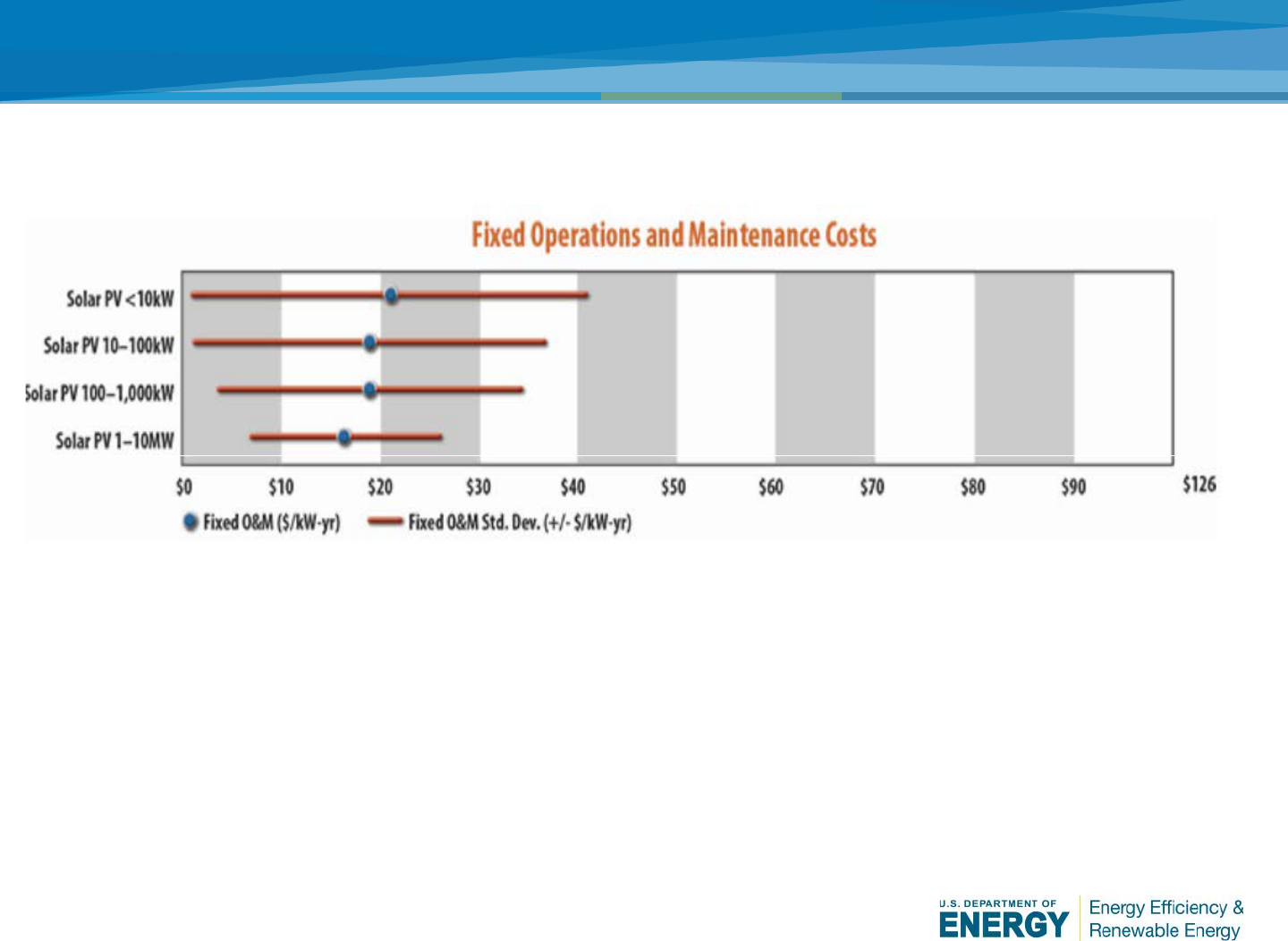
Heuristic PV O&M Costs
Source: FEMP Cost and Performance Matrix , http://www.nrel.gov/analysis/tech_cost_om_dg.html
Annual Technology Baseline, http://www.nrel.gov/docs/fy16osti/66944.pdf
NREL Annual Technology Baseline
• $16.7/kWDC/yr for Utility-Scale
• $20/kWDC/yr for Residential
There is a wide range in the reported data from $0 to $110/kW/year
Often a single annual value is reported per kW or per kWh.

4
The PV O&M Working Group concentrated on three estimates
related to the cost of delivering a PV O&M Program:
o Annual Cash Flows
o Net Present Value, LCOE
o Reserve Account
The working group has developed a PV O&M Cost Model that can
be used to estimate O&M costs.
Estimating PV O&M Costs

5
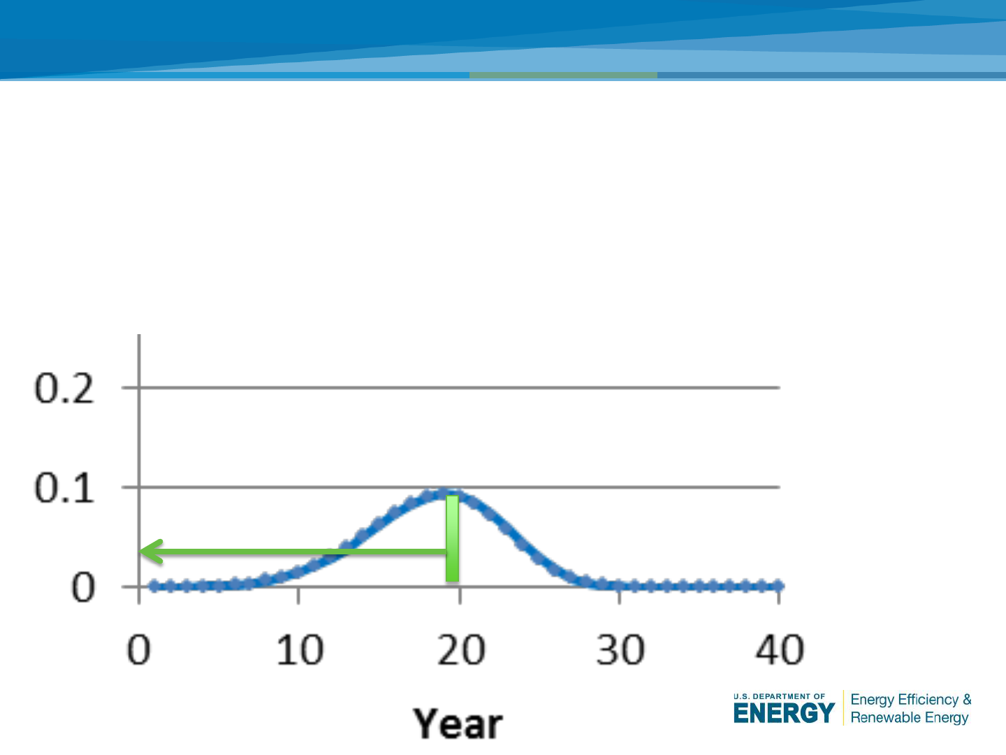
Weibull Failure Distribution
Q, the probability that a component will fail in any given year, y, is
calculated according to the Weibull probability density function.
The equation for the Weibull probability density function is:
=
(−1)
(
−
)
α = the “shape factor” of the distribution, indicating how spread out the probability of
failure is over the years,
β = the “scale factor” of the distribution, indicating over which years of the analysis
period the bulk of the failure distribution lies.
Parameters, α and β, are obtained from heuristic failure data
PV ROM database of failure and reliability data; Sandia National Laboratory.
Source: http://reliawiki.org/index.php/The_Weibull_Distribution
MS Excel function
=WEIBULL.DIST(y,α,β,FALSE).
6
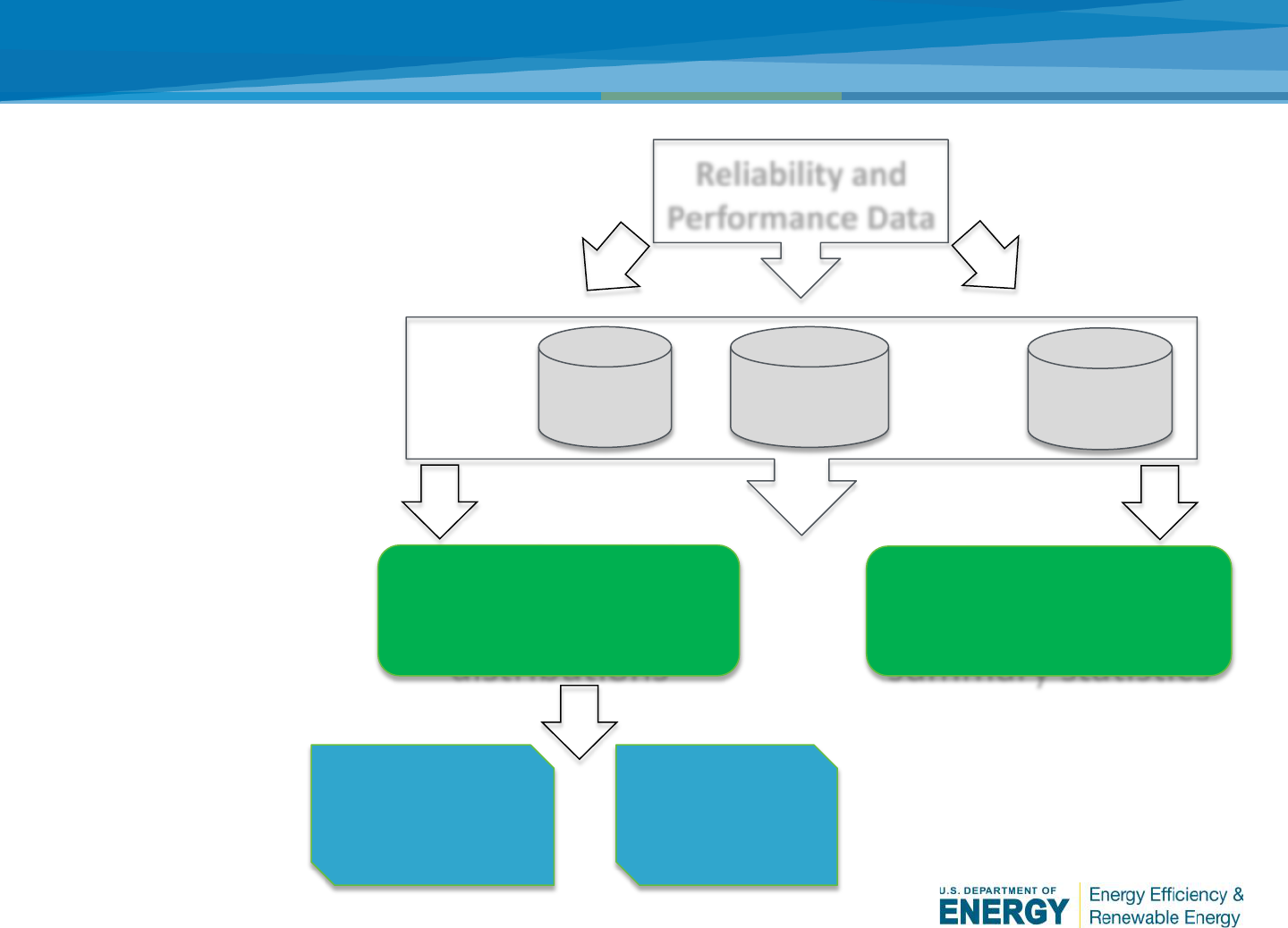
Sandia’s General Process for Evaluating Reliability Impacts
PVROM
Event
Database
Event
Logs
Data
Collection &
Storage
Sandia
Provided
Owner
Provided
Data
Analysis
Reliasoft tools for
reliability
distributions
Other tools for
reliability data
summary statistics
PV O&M
Cost Model
Data
Application
and Further
Analysis
PV
Performance
Model
Raw Data
Generation
Reliability and
Performance Data
Source: Geoff Klise, Sandia National Laboratories
7
Net Present Value of Replacement Cost
Q=failure probability
Replacement cost inflated to year t
Discounted to
present value
C
replacement
= Cost to replace Component in year 1
Q= probability of failure of component in each year t
d=discount rate (%/year)
i=inflation rate (%/year)
t=number of year
Present Value=C
replacement
x Q x (1+i)^t / (1+d)^t

8
Calculation of Reserve Account - Background
• Weibull distribution of failure gives us a good estimate of life-cycle
cost and levelized cost of energy (LCOE), but the method spreads
the costs over the years and show a rather uniform average cost
per year.
• Financiers are asking for a tool that calculates “maximum
exposure”; in other words, what dollar amount of a “reserve
account” or “line of credit” would a bank offer to sell to a
project?”
• Reserve account is calculated for each year of the analysis period.

9
Definition of Terms
• P= the probability that a component will not fail in any
giv
en year, specific to that year only according to the
Weibull distribution of component failure.
• Q= the probability that a component will fail in the same
y
ear;
• (P+Q)=1
• R= the desired probability that the reserve account will
be
sufficient to pay for required replacements in that
year.
• N=the number of a certain type of component (for
ex
ample N=10 inverters, N=500 combiner boxes, or
N=50,000 PV modules)

10
Start With a Simple Example…
Consider two inverters:
N=2
Replacement Cost (Year 1):
C
replacement
=$10,000 each
Weibull Failure Distribution:
Mean Interval (years) β=20
Shape Factor α=5.0
In year 20:
P = probability of non-failure
P = 0.908
Q = probability of failure
Q = 0.092
Weibull distribution
=WEIBULL.DIST (Year, Shape Factor, Mean Interval)

11
Mind Your P’s and Q’s…
• Spare in Reserve for NEITHER of the two inverters:
Reserve Account: $0
P
1
P
2 =
P^N=(0.908)^2=0.824 (you get this level of
availability for free)
• Spare in Reserve for EITHER ONE of the two inverters:
Reserve Account=$10,000
P
1
P
2 +
P
1
Q
2
+ P
2
Q
1
= 0.824+(0.908*0.092)* 2 =0.991
• Spares in reserve for BOTH of the inverters:
Reserve Account= $20,000
P
1
P
2 +
P
1
Q
2
+ P
2
Q
1
+ Q
1
Q
2
=0.824+0.300+ (0.092)^2=1.00
• So in this simple example; the result would be “within a
99.1% chance your maximum exposure any year will be less
than the cost of one inverter”, or $10,000.
• Notice that if we raise the desired probability from 0.99 to
0.999 (three nines), then our maximum exposure would be
the cost of two inverters in the year, or $20,000.
• The cost model is coded such that the desired probability is
an input, with a default of 0.95, and the calculation returns
the required amount of Reserve Account
Desired
Probability
that
Reserve
Account is
Sufficient
Reserve
Account
0.824 $0
0.991 $10,000
1.000 $20,000

12
General Polynomial Expansion
Binomial Theorem, 1666, Sir Isaac Newton
(
P+Q)=1
Total number of components = N
Number of components funded in reserve account=n
(
P+Q)
N
= 1
P
N
+ NP
N-1
Q + N(N-1)P
N-2
Q
2
/2! +….+ Q
N
=1
Add
up the first n+1 terms to find the probability that n components will be
operational (1<n<N).
Polynomial Expansion form changes with N, and computationally intense to
evaluate at large values of N
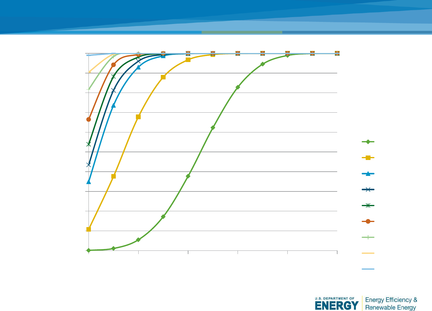
13
Reserve account graph
0
0.1
0.2
0.3
0.4
0.5
0.6
0.7
0.8
0.9
1
0 0.2 0.4 0.6 0.8 1
R=probability that reserve account will be
sufficient to cover replacements of a
component
n/N=fraction of total number of a component covered by reserve
account
0.5
0.2
0.1
0.08
0.06
0.04
0.02
0.01
0.001
Q=Probability
that each of a
component will
fail in a given
year; from failure
distribution

14
Example Calculation of Reserve Account
In this example we consider 10 components, each with a replacement cost of $1000 in a
given year, and with a Weibull failure probability of Q=0.05 in this given year.
The desired probability that the reserve account will be sufficient is R=0.999 (99.9%
certainty).
INPUTS
N= 10
C
replacement
= $1,000
Q= 0.05
R= 0.999
OUTPUTS
Required n/N=0.303 (required fraction of total number of component covered by
reserve account in order to achieve desired probability that reserve account will be
sufficient in a given year)
C reserve account = $3,030 (amount in reserve account for this type of component in
this given year)
The resulting dollar amount to keep in
the reserve account to cover failure of
this component in the given year is
(0.303)*(10)*($1000) or $3,030.

15
Implementation of NPV and Reserve Account in Cost Model
Inputs
Number of Inverters: 2
Replacement Cost (each): $10,000
Desired Confidence that Reserve
Account Sufficient: 0.900000
Mean Interval (years): 20.00
Weibull Shape Factor: 5.00
Analysis Period: 25 years
Discount Rate: 7.00% per annum
Inflation Rate: 2.00% per annum
Continue example of two inverters
Outputs
Net Present Value of Replacement Costs $8,284
Maximum Amount Reserve Account $10,501 in year 20

16
Calculation of Net Present Value and Reserve Account
• Annual Cost and Reserve Account both modified by:
o Within analysis period?
o Within warranty period?...type of warranty?
o Fixed interval or Weibull distribution?
o Yearly inflation of costs.
• This is done for each measure in the PV O&M Cost Model (PV
module replacement, inverter replacement…all) and added up to
calculate the total amount in the Reserve Account for each year of
the Analysis Period.
17
18
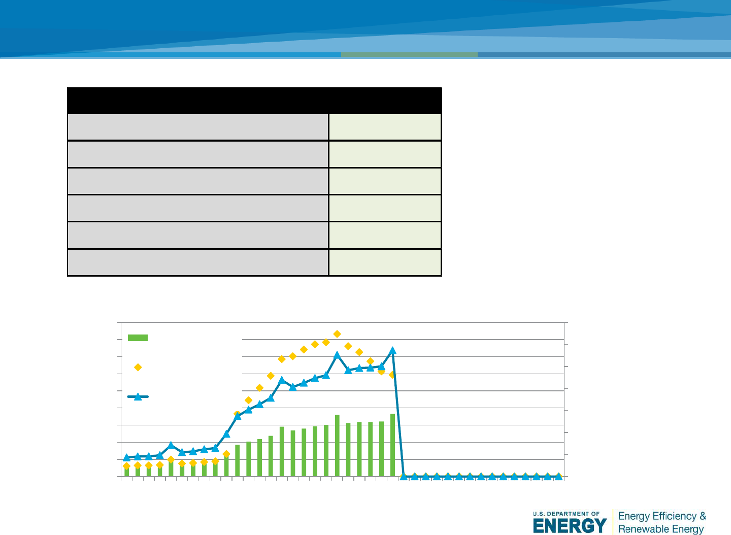
PV O&M Cost Model Results
Results
Annualized O&M Costs ($/year)
$126,471
Annualized Unit O&M Costs ($/kW/year)
$12.65
Maximum Reserve Account
$831,685
Net Present Value O&M Costs (project life
$1,800,124
Net Present Value (project life) per Wp
$0.180
NPV Annual O&M Cost per kWh
$0.011
$0.000
$0.005
$0.010
$0.015
$0.020
$0.025
$0.030
$0.035
$0
$100,000
$200,000
$300,000
$400,000
$500,000
$600,000
$700,000
$800,000
$900,000
1 3 5 7 9 11 13 15 17 19 21 23 25 27 29 31 33 35 37 39
LCOE ($/kWh)
Annual Cash Flow ($/year)
Year
Annual Cash Flow
Reserve Account
LCOE ($/kWh)

19
High LCOE in Late Performance Period
• Warranties have expired
• Inflation has raised parts and labor prices
• The Weibull failure distributions show high failure rates
in
later years
• The performance had degraded (0.5%/year)
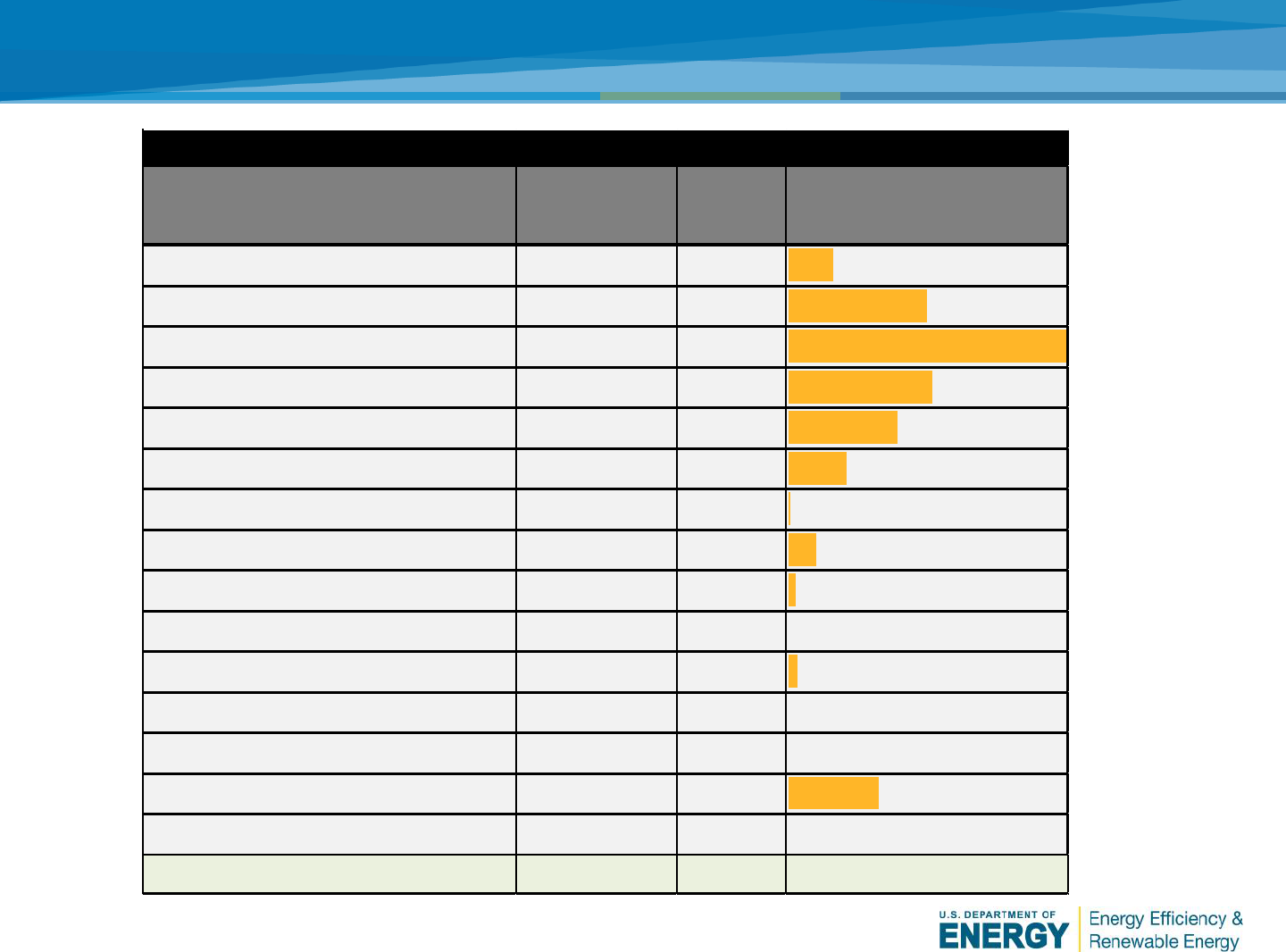
Results by Component
Service Avg. Cost/Yr NPV (Life) % of Total
Administrator $8,139 $88,635 5%
Cleaner $25,239 $274,892 15%
Inverter specialist $71,551 $550,944 31%
Inspector $26,850 $286,646 16%
Journeyman electrician $29,261 $216,399 12%
PV module/array Specialist $14,563 $114,939 6%
Network/IT $186 $1,825 0%
Master electrician $7,223 $53,383 3%
Mechanic $2,132 $14,926 1%
Designer $0 $0 0%
Pest control $1,702 $18,536 1%
Roofing $0 $0 0%
Structural engineer $10 $69 0%
Mower/Trimmer $16,424 $178,884 10%
Utilities locator $6 $44 0%
Total $203,285 $1,800,124 100%
Lifetime NPV by Service Type
21
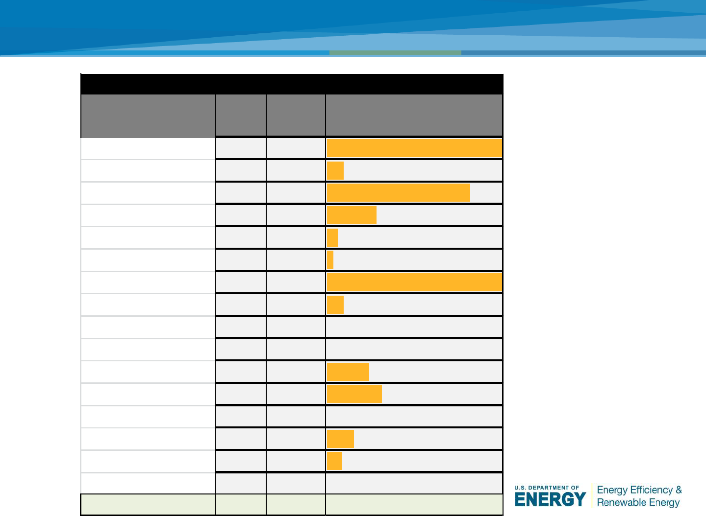
Results by Service Provider
Component
Avg.
Cost/Yr NPV (Life) % of Total
AC wiring $2,423 $22,299 1%
Asset Management $4,797 $52,249 3%
Cleaning/Veg $41,644 $453,566 25%
DC wiring $19,160 $158,395 9%
Documents $3,286 $35,784 2%
Electrical $1,894 $20,351 1%
Inverter $72,075 $555,708 31%
Mechanical $5,607 $53,304 3%
Meter $19 $205 0%
Monitoring $72 $783 0%
PV Array $12,517 $135,644 8%
PV module $25,036 $175,764 10%
Roof $0 $0 0%
Tracker $7,960 $86,694 5%
Transformer $6,795 $49,377 3%
(blank) $0 $0 0%
Total $203,285 $1,800,124 100%
Lifetime NPV by Component Type

22
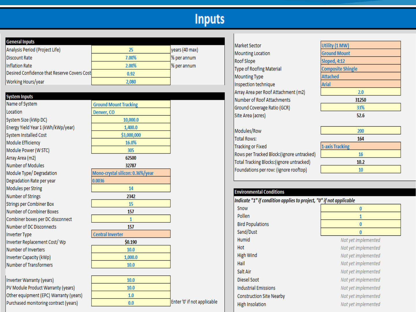
PV O&M Cost Model Example: 10 MW ground-mount
$0
$50,000
$100,000
$150,000
$200,000
$250,000
$300,000
$350,000
$400,000
$450,000
1 2 3 4 5 6 7 8 9 10 11 12 13 14 15 16 17 18 19 20 21 22 23 24 25
Annual O&M Expense ($)
Year
Operations administration (planned)
Inverter replacement reserve (corrective)
Module replacement reserve (corrective)
Component parts replacement (Planned)
System inspection and monitoring (Planned)
Module cleaning and vegetation management
(Planned)
Mike’s Category
Annual $/kW
Component parts replacement (Planned)
$0.58
Inverter replacement reserve (corrective)
$3.84
Module cleaning and vegetation management (Planned)
$3.25
Module replacement reserve (corrective)
$0.91
Operations administration (planned)
$2.80
System inspection and monitoring (Planned)
$1.71
TOTAL
$13.09

23
• Asset Management Software
o Benchmarking performance
o Continuous Performance Index
o Curation and Quality Control on Data
o Efficient business transactions; lower cost
o Improved analytics
o Knowledge management-diagnostics and troubleshooting
o Keep track of preventative maintenance requirements
o Calculate predictive or condition-based maintenance.
Recommendations for Cost Reductions

Recommendations for Cost Reductions
Warranty management practices
• Do not void warranty b
y mishandling
or not observing instructions or
conditions of the warranty.
• Curate data to prove th
at a module
is underperforming,
• Plan for labor t
o remove, ship, and
re-install an underperforming
module.
• Try to get a warranty for the
ma
nufacturer to “repair or replace”
rather than “supplement,”
• Consider Insura
nce Backed
Guarantee (IBG) that provides that
warranty claims will still be processed
in the event of the liquidation,
receivership, or closure of a dealer
Failure to follow “product box handling and
storage requirements” can cause damage when
moved and void a warranty
Photo by Andy Walker, NREL
25
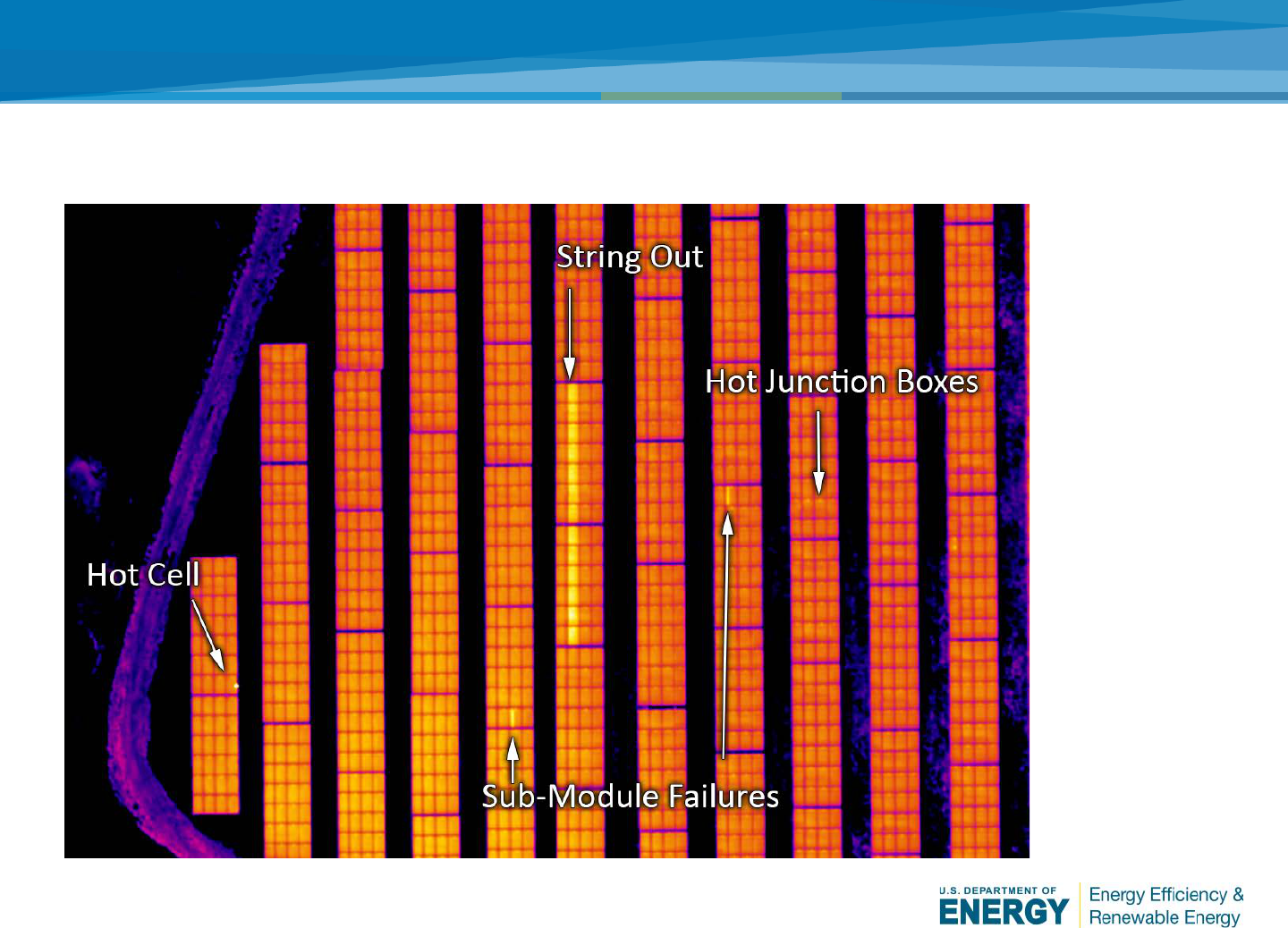
• Remote imaging, Aerial Inspection
Recommendations for Cost Reductions
Image by Rob Andrews, Heliolytics

26
• O&M Business Models
o “The UBER of PV O&M”
o O&M Cooperative business structures
o Shared facilities and inventories
• Module-level power electronics
o Reduced production losses
o Covers rapid shutdown requirements
o Detailed data
o Conventional AC wiring
• Standardization of parts, suppliers, procedures
o Optimized reserve
o Remove obsolete inventory and reduce inventory exceeding
the maximum stocking level to reduce cost to count, move,
store, secure, insure and taxes.
Recommendations for Cost Reductions

Thank You!
