
Conguration Guide | PUBLIC
Document Version: 1.1–2023-02-17
Model Conguration Guide
SAP Integrated Business Planning for Supply Chain 2302
© 2023 SAP SE or an SAP aliate company. All rights reserved.
THE BEST RUN
Content
1 Document History........................................................... 8
2 About This Guide............................................................9
3 Planning Models in SAP Integrated Business Planning...............................10
4 Attributes.................................................................13
4.1 Creating Attributes...........................................................13
4.2 Attribute Congurations....................................................... 15
4.3 Extending the Length of an Attribute...............................................16
4.4 Editing Attributes............................................................ 17
4.5 Deleting an Attribute..........................................................19
5 Master Data Types.......................................................... 21
5.1 Description Attributes.........................................................23
5.2 Copy Options for Master Data Types...............................................23
5.3 Creating Simple Master Data Types...............................................24
5.4 Creating Attribute Checks......................................................26
5.5 Creating Compound Master Data Types............................................28
5.6 Creating External Master Data Types.............................................. 29
5.7 Creating Reference Master Data Types............................................. 31
Filtering Reference Master Data Types...........................................32
5.8 Creating Virtual Master Data Types................................................34
5.9 Master Data Type Congurations.................................................36
5.10 Change of a Master Data Type...................................................37
5.11 Deletion of a Master Data Type...................................................40
5.12 Tracking Changes to Personal Master Data.......................................... 41
6 Time Proles and Time Periods................................................ 43
6.1 PERIODID and PERIODID(n) Attributes in Time Prole Levels.............................44
6.2 Creating Time Proles.........................................................44
6.3 Options for Creating Time Periods................................................46
6.4 Creating Time Periods from a Template.............................................47
6.5 Creating Time Periods with an Application Job....................................... 48
6.6 Change and Deletion of Time Proles..............................................49
6.7 Conguring Aggregation and Disaggregation of Data Across Dierent Time Prole Levels......... 51
7 Planning Areas.............................................................54
7.1 Sample Planning Areas........................................................56
2
PUBLIC
Model Conguration Guide
Content
7.2 Options for Creating a Planning Area...............................................61
7.3 Creating a Planning Area by Copying a Sample Planning Area.............................62
Create New with Dependencies................................................64
Create New by Partial Copy...................................................67
7.4 Creating a Planning Area in the Planning Areas App....................................69
7.5 Creating a Planning Area by Copying a Non-Sample Planning Area..........................71
7.6 Assigning Attributes to a Planning Area.............................................72
7.7 Assigning an Attribute Category to a Planning Area Attribute............................. 74
7.8 Replacing the Time Prole in a Planning Area.........................................77
7.9 Updating a Planning Area with Content from Another Planning Area........................80
Replace Existing...........................................................81
Replace Existing Including Dependencies.........................................82
Merge with Existing........................................................84
Partial Merge.............................................................88
7.10 Using Multiple Planning Areas...................................................95
7.11 Downloading a Planning Area....................................................97
7.12 Uploading a Planning Area......................................................99
7.13 Comparing Planning Areas.....................................................100
7.14 Deleting a Planning Area...................................................... 102
8 Planning Levels............................................................104
8.1 Creating Planning Levels......................................................106
8.2 Assigning Attributes to Planning Levels ........................................... 109
8.3 User-Dened Source Assignment for Planning Level Attributes............................111
Example Use Case........................................................ 112
Creating the Source Assignment.............................................. 113
Modeling Requirements for Source Assignment....................................114
8.4 Change and Deletion of Planning Levels............................................115
8.5 Controlling Planning Objects....................................................116
9 Attributes as Key Figures....................................................120
9.1 Dening an Attribute as a Key Figure..............................................130
9.2 Troubleshooting for Attributes as Key Figures........................................132
10 Key Figures...............................................................135
10.1 Types of Key Figures......................................................... 135
10.2 Creating Key Figures.........................................................138
Conguration of Key Figure Fixing............................................. 147
Enabling Planning Notes for a Key Figure........................................ 149
Conguration of Proportional Disaggregation.....................................150
Conversion Conguration................................................... 151
10.3 Copying Key Figures......................................................... 152
Model Conguration Guide
Content
PUBLIC 3
10.4 Editing Key Figures.......................................................... 153
10.5 Creating External Key Figures...................................................154
10.6 Decimal Places in Key Figure Values.............................................. 155
10.7 Distance of Key Figures from Their Data Sources .....................................156
11 Key Figure Calculations..................................................... 158
11.1 Adding Calculations to Key Figures...............................................158
11.2 Calculation Graphs..........................................................160
11.3 Commonly Used Functions and Expressions........................................ 162
11.4 MIN and MAX with Multiple Inputs............................................... 169
11.5 COUNT...................................................................170
11.6 STDDEV..................................................................172
11.7 Stored Key Figure Calculation...................................................173
11.8 Calculations at Request Level...................................................174
11.9 Calculations Across Dierent Planning Levels........................................175
11.10 Defaulting to Another Key Figure.................................................177
11.11 Simplied Key Figure Calculations................................................179
Cumulative Aggregation....................................................180
Last Period Aggregation....................................................192
Rolling Aggregation....................................................... 196
Dynamic Rolling Aggregation.................................................199
Period Shift.............................................................205
Weighted Average........................................................ 210
Coverage...............................................................215
Calendar...............................................................235
Generate Missing Time Periods...............................................239
Last Value Calculation.....................................................248
Current Value Calculation...................................................251
Window-Based Aggregation.................................................254
11.12 Using Attributes in Key Figure Calculations.........................................258
11.13 Using Time Periods in Key Figure Calculations.......................................259
11.14 Exceeding the 12-Digit Integer and 6-Digit Decimal Limit in Key Figure Calculations............ 260
12 Dening Key Figure Groups.................................................. 263
13 Business Meaning..........................................................265
14 Creating Versions..........................................................266
15 Planning Operators........................................................ 268
15.1 Assigning a Planning Operator to a Planning Area.....................................272
15.2 Advanced Simulation Operator..................................................272
Advanced Simulation Proles................................................ 274
4
PUBLIC
Model Conguration Guide
Content
15.3 Copy Operator (Advanced).................................................... 275
Copy Operator Proles.....................................................276
Processing of Key Figures...................................................278
Example Settings for Key Figure Selection....................................... 281
Example: Dierent Options for Value-Based Filter..................................282
15.4 Snapshot (SNAPSHOT) Operator................................................283
15.5 Redo Snapshot (SNAPSHOTREDO) Operator....................................... 283
15.6 Inventory Optimization (IO) Operator.............................................284
16 Conguring Original Snapshots...............................................287
17 Activating Planning Models...................................................291
17.1 Statuses of Model Entities.....................................................292
Example: Changing Model Entities That Are Dependent on Each Other...................295
Example: Deleting an Attribute from an Active Master Data Type and Active Planning Area
.....................................................................300
17.2 Activating Time Proles.......................................................303
17.3 Activating Master Data Types...................................................304
17.4 Activating Planning Areas.....................................................306
Activating Planning Areas in the Planning Areas App................................308
Enhanced Version of Planning Area Activation.....................................310
Application-Specic Checks for Planning Area Activation.............................311
Suppressing Errors and Activating the Planning Area with Limited Scope..................312
17.5 Deleting Active Objects (Active Deletion)...........................................312
Troubleshooting for Active Deletion............................................314
18 Modeling Requirements (Checks and Errors)..................................... 316
18.1 Time Proles...............................................................316
18.2 Master Data Types...........................................................318
18.3 Planning Areas.............................................................322
18.4 Planning Levels.............................................................326
18.5 Key Figures............................................................... 327
18.6 Suppressible Errors......................................................... 339
19 Restore Active Instance..................................................... 341
19.1 Restore Active Instance for Planning Areas......................................... 341
19.2 Restore Active Instance for Other Entities..........................................342
19.3 Restore Active Instance After Copy...............................................344
20 Historical States of Model Entities.............................................346
20.1 Viewing Historical States......................................................346
20.2 Restoring a Historical State of a Planning Area.......................................348
20.3 Archiving a Historical State of a Planning Area.......................................349
Model Conguration Guide
Content
PUBLIC 5
21 Setting Up Multilanguage Support for Modeling Objects............................350
22 Export and Import of Software Collections.......................................352
22.1 Export and Import of Extension Items in Your System Landscape.........................360
22.2 Best Practices for Exporting Planning Models.......................................363
22.3 Exporting Planning Areas in a 2-Phase Conguration Project.............................365
23 Emergency Access to Production System ....................................... 368
24 Reason Codes.............................................................369
24.1 Creating Reason Codes.......................................................369
25 Global Conguration....................................................... 370
25.1 Managing Global Conguration Parameters.........................................370
25.2 Global Conguration Parameters................................................ 371
26 Conguration History.......................................................431
27 Advanced Modeling Topics...................................................433
27.1 Time-Independent Key Figures..................................................433
27.2 Conguring Currency Conversion................................................434
27.3 Conguring Unit of Measure Conversion...........................................436
27.4 Attribute Transformations.....................................................438
27.5 Weighted Average Calculation.................................................. 441
27.6 Conguring Price and Cost for Currency and UoM Conversions...........................443
27.7 Split Factor Calculation.......................................................445
27.8 How to Enable the Change History?..............................................446
Enabling the Change History for Planning Areas...................................448
Enabling the Change History for Key Figures......................................449
Enabling Users to View the Change History...................................... 450
Optional Settings for the Change History........................................ 451
27.9 Setting up Change-History-Based Calculations......................................452
Enabling Change-History-Based Calculations.....................................453
Conguring History-Dependent Key Figure Calculations.............................455
Activation of a Planning Area Congured for Change-History-Based Calculations............456
27.10 Conguring Period-to-Period Comparison with Time Prole Attributes......................457
28 Naming Conventions of Model Entities......................................... 460
28.1 Reserved Names and Naming Restrictions..........................................461
28.2 How to Create a Key Figure with the ID of a Deleted Attribute or an Attribute with the ID of a
Deleted Key Figure..........................................................463
29 Monitoring and Troubleshooting.............................................. 465
29.1 Simulate Key Figure Calculations ................................................465
How to Use the App?......................................................466
6
PUBLIC
Model Conguration Guide
Content
Example: Missing Exchange Rates.............................................467
Example: Division by Zero...................................................470
Filter Blocks in Simulation...................................................470
Handling of Missing Input...................................................471
Changing Key Figure Values Manually for Simulations...............................473
Limitations in the Simulate Key Figure Calculations App............................. 474
29.2 Where-Used Graphs......................................................... 474
29.3 Analyze Data Volume in Calculations..............................................476
What Is a Data Volume Report?...............................................477
What Happens When Running the Report?.......................................477
How to Interpret the Results of the Report?...................................... 478
What's Next?............................................................481
29.4 Filter Blocks...............................................................482
Example: Time Attribute Transformation........................................485
Example: Master Data Attribute Transformation...................................488
Example: Cumulative Aggregation.............................................491
Watch a video!...........................................................493
Model Conguration Guide
Content
PUBLIC 7

1 Document History
Note
Until three months after the publication of a new release of SAP Integrated Business Planning for Supply
Chain, we publish regular documentation updates on the SAP Help Portal. If you use a local PDF copy
or a paper printout of this document, make sure that you have the latest version. You can nd it at http://
help.sap.com/ibp2302.
The following table provides an overview of the most important document changes.
Version Date Description
1.1 2023-02-17 The following changes have been made:
• The Importing a Software Collec
tion to the P-System section has
been enhanced with information
about transport automation.
• Outdated information about mutu
ally assigned description attributes
has been removed from the De
scription Attributes section.
• The Creating Attribute Checks sec
tion has been enhanced with infor
mation related to copying the mas
ter data type with the Copy Version
application job template.
1.0 2023-02-03 Initial version for SAP Integrated Busi
ness Planning for Supply Chain 2302
8 PUBLIC
Model Conguration Guide
Document History

2 About This Guide
SAP Integrated Business Planning provides extensive functions for creating, updating, and capturing
information in a plan, which is congured using a planning model.
This model conguration guide is aimed at expert business users, consultants, and others who are creating,
changing, or extending a company planning model. Based on the Web user interface that is used to congure
the planning model, the guide provides task-based information to help you carry out common modeling tasks,
such as:
• Creating master data types and attributes, time proles, planning areas, planning levels, key gures
(including calculations), versions, and planning operators
• Activating, copying, exporting, and importing a planning model
• Managing reason codes and global conguration parameters
• Setting up multilanguage support for the supported modeling object types
The guide also introduces some advanced modeling concepts, such as modeling for currency conversion and
for unit of measure conversion and for attribute transformations.
Note
The guide contains many examples to illustrate modeling tasks and concepts. To make it easier for you
to follow the examples, they have been based, wherever possible, on the SAPIBP1 sample planning area,
which is delivered with SAP Integrated Business Planning.
Based on your planning model, you can create planning views and work on your data using the SAP Integrated
Business Planning, add-in for Microsoft Excel. For more information, see the SAP Help Portal at http://
help.sap.com/ibp , under Application Help User Interface Planning with Microsoft Excel .
Model Conguration Guide
About This Guide
PUBLIC 9

3 Planning Models in SAP Integrated
Business Planning
A planning model describes the structure of your plan in terms of data and calculations. It denes how data is
stored, calculated, and aggregated in the system. From a technical perspective, a planning model is a collection
of master data and time series data that is organized in dimensions and enhanced with specic calculations. All
models are based on the following entities:
• Attributes
• Master data types
• Time proles
• Planning areas
• Planning levels
• Key gures (including snapshots)
• Versions
• Calculations
• Miscellaneous additional entities such as global conguration parameters, planning operators, and reason
codes.
The gure below illustrates the relationship between the main conguration entities.
10
PUBLIC
Model Conguration Guide
Planning Models in SAP Integrated Business Planning

The entities shown in the gure are explained in the following table:
Main Conguration Entities
Entity Explanation
Common entities Attributes, master data types , and time proles must be
dened in SAP IBP. They are available for use in any planning
area.
Attributes Attributes describe an individual eld and data type that is
used in the planning model. The product ID is an example for
an attribute.
Master data types Master data types are groupings of attributes. For example,
a master data type could group all attributes belonging to
the product, such as product ID, product group, and so on.
A master data type can be assigned to multiple planning
areas, and a planning area has multiple master data types
assigned.
Time proles The time periods in which planning data can be managed
(for example, weekly, monthly, and so on) and the hierarchy
of these time periods make up a time prole. A time prole
can be assigned to multiple planning areas. A planning area
has exactly one time prole assigned.
Planning areas Planning areas are structures consuming the elements re
quired in the planning process (attributes, master data
types, time proles). The elements are selected specically,
for example, for demand planning. (At this stage, the plan
ning area is still lacking planning levels and key gures.)
Planning levels For each planning area, one or more planning levels are de
ned. A planning level is a combination of attributes option
ally plus a time period. For example, a planning level may
consist of customer ID, location ID, and product ID with an
associated time period, for example, weekly.
Key gures On each planning level, key gures are congured. For exam
ple, the key gure consensus demand could be congured
on the level of customer ID, location ID, product ID, and a
weekly time period. It represents the consensus demand
quantity of a specic product, delivered to a specic cus
tomer, from a specic location, in a specic calendar week.
Baseline version After the key gure conguration, the planning area is com
pletely congured and a baseline version is automatically
generated.
Model Conguration Guide
Planning Models in SAP Integrated Business Planning
PUBLIC 11

Entity Explanation
Versions Apart from the baseline version, a planning area can have
other versions. These can include only a subset of key g-
ures, for example, because you do not want all users to see
all the data. Versions can also be used to represent optimis
tic or pessimistic plans by using more optimistic or more
pessimistic key gure values.
Planning operators are functions that are associated with a planning area. An important example of a planning
operator is the Copy Operator (Advanced) operator, which you can use to copy key gure values within a
planning area or between two planning areas.
SAP Integrated Business Planning for Supply Chain (SAP IBP) allows you to congure and customize your own
planning models to address your unique business requirements. The following apps, which you can access
from the launchpad, include all features that enable you to congure a model from scratch, and activate it:
• Attributes
• Master Data Types
• Time Proles
• Reason Codes
• Time Proles
• Sample Model Entities
• Planning Areas
Many model entities (planning areas, master data types, and time proles) can also be copied and modied.
(You cannot, however, copy attributes or planning operators.)
12
PUBLIC
Model Conguration Guide
Planning Models in SAP Integrated Business Planning

4 Attributes
Attributes are characteristics of master data types, for example, an attribute of the customer master data type
might be country or region. Attributes can be either numeric or non-numeric.
The following data types are supported for attributes:
• nvarchar
• decimal
• integer
• timestamp
Note
You can only use decimal attributes as key gures in the planning area, and not as planning area dimension
attributes.
To support the planning calendar function of SAP Integrated Business Planning, special attribute types are
available with xed properties as follows:
• Calendar attribute:
• Data type: NVARCHAR
• Length: 32
• Time zone attribute:
• Data type: NVARCHAR
• Length: 6
4.1 Creating Attributes
Use the Attributes app to create attributes.
Prerequisites
Make sure you have the necessary authorizations for this activity, that is, the business catalogs required for
this activity are assigned to a business role that is assigned to your business user. For more information see the
SAP Help Portal at
http://help.sap.com/ibp, under Application Help for SAP Integrated Business Planning
Identity and Access Management Basic Concepts Business Catalogs .
Model Conguration Guide
Attributes
PUBLIC 13

Procedure
1. In the Attributes app, choose New. To create special attribute types (calendar or time zone attributes),
select the attribute type from the dropdown next to the New button.
You can also create the attributes in the Master Data Types app. You can display, edit, and delete the
attributes in the Attributes app, regardless of where you created them.
2. In the New Attribute dialog provide the details for the attribute.
To create the product ID attribute, you could enter the following:
• Attribute ID: S2PRDID
Caution
We use the sample model entities in many examples throughout the user assistance for SAP IBP. In
general, you have the freedom to customize the model entities according to your business needs.
However, to run the inventory operators and time-series-based supply planning algorithms, you
have to use specic technical IDs dened by SAP for the relevant master data types, attributes,
and key gures. For demand sensing, the same applies to certain master data attributes and key
gures for which a business meaning has not been specied.
For more information, see the documentation of the relevant planning operator in this guide and
the respective chapter of the application help.
• Name: Product ID
• Description: Product Identier
• Data Type: NVARCHAR
• Length: 40
Caution
Make sure that the ID you specify for the attribute does not exist in any of the SAP sample planning
areas. An attribute with the same ID as an attribute in an SAP sample planning area can be overwritten
if you copy the SAP sample planning area.
Note
The length of an attribute must not exceed 450 characters. Attributes longer than that cannot be
shown in a planning view and cannot be used in attribute-based lters in the SAP Integrated Business
Planning, add-in for Microsoft Excel or in Planner Workspaces. Attributes longer than 450 characters
should be modelled as description attributes (e.g. Product Description as a description attribute of
Product ID).
3. Save your entries.
Related Information
How to Create a Key Figure with the ID of a Deleted Attribute or an Attribute with the ID of a Deleted Key Figure
[page 463]
14
PUBLIC
Model Conguration Guide
Attributes

Attribute Congurations [page 15]
Creating Simple Master Data Types [page 24]
Creating Compound Master Data Types [page 28]
Creating Reference Master Data Types [page 31]
Attributes [page 13]
4.2 Attribute Congurations
Specic settings for creating attributes.
Attribute Congurations
ID Description Data Type Length
S2CURRID
Currency ID NVARCHAR 5
S2CURRDESC
Currency Description NVARCHAR 60
S2CURRTOID
Currency To ID NVARCHAR 5
S2CURRTODESC
Currency To Description NVARCHAR 60
S2CUSTDESC
Customer Description NVARCHAR 60
S2CUSTID
Customer ID NVARCHAR 20
S2DISCTCHANNEL
Distribution Channel NVARCHAR 2
S2LOCDESC
Location Description NVARCHAR 60
S2LOCID
Location ID NVARCHAR 20
S2LOCTYPE
Location Type NVARCHAR 10
S2ORDERQTY
Cumulative Order Quantity in
Sales Units
DECIMAL(18,6) -
S2PRDDESC
Product Description NVARCHAR 60
S2PRDFAMILY
Product Family ID NVARCHAR 40
S2PRDFAMILYDESCR
Product Family Description NVARCHAR 60
S2PRDID
Product ID NVARCHAR 40
S2SALESDOC
Sales Order NVARCHAR 10
S2SALESITEM
Sales Order Item NVARCHAR 10
Model Conguration Guide
Attributes
PUBLIC 15

Related Information
Creating Attributes [page 13]
Attributes [page 13]
4.3 Extending the Length of an Attribute
Prerequisites
Make sure you have the necessary authorizations for this activity, that is, the business catalogs required for
this activity are assigned to a business role that is assigned to your business user. For more information see the
SAP Help Portal at
http://help.sap.com/ibp, under Application Help for SAP Integrated Business Planning
Identity and Access Management Basic Concepts Business Catalogs .
Context
You can extend the length of an attribute up to 450 characters. Attributes longer than that cannot be shown in
a planning view and cannot be used in attribute-based lters in the SAP Integrated Business Planning, add-in
for Microsoft Excel or in Planner Workspaces. Attributes longer than 450 characters should be modelled as
description attributes.
If you extend the length of an attribute, you must make sure that all model entities that use the attribute are
updated with the new length. You must activate the relevant master data types, time proles, and planning
areas again for the changes to take eect, to keep the database consistent, and to prevent runtime errors.
Note
If you use an attribute, which is used in an SAP sample planning area, in any of your planning areas, and the
length of this attribute has been changed in the SAP sample planning area, an advanced copy of the SAP
sample planning area overwrites the attribute length in your planning areas. You must activate the time
proles, master data types, and planning areas that use this attribute again. After activation, the attribute
will have the new length consistently for all model entities where it is used.
Note
Please note that calendar attributes and time zone attributes have a xed length, which cannot be changed.
Caution
Please also note that you cannot change the length of an attribute in planning areas for order-based
planning, the length must remain as dened in the SAP7 and SAP7F sample planning areas.
16
PUBLIC
Model Conguration Guide
Attributes

Procedure
1. In the Attributes app, change the length of the attribute.
2. Find the time proles, master data types, and planning areas that use the attribute you have changed.
To do this, click the numbers in the corresponding cells in the Attributes app.
3. Activate the time proles that use the attribute you have changed.
4. Activate the master data types that use the attribute you have changed.
5. Activate the planning areas that use the attribute you have changed.
Related Information
Activating Time Proles [page 303]
Activating Master Data Types [page 304]
Activating Planning Areas [page 308]
Updating a Planning Area with Content from Another Planning Area [page 80]
4.4 Editing Attributes
You may want to change an attribute. However, you’ll nd that not all elds of an attribute are available for
editing. The changes you can do depend on the following factors:
• If the status of the attribute is active or inactive
• If the attribute is used in higher-level entities, for example, in master data types, and planning areas
• If master data records exists for one or more master data types that use the attribute
You can change any eld of an attribute that you have never activated (that is, only an inactive instance of the
attribute exists). You can also delete the attribute.
If an attribute has already been activated with a master data type (even if the attribute currently has an inactive
instance), certain rules apply for which elds or parameters you can change or delete.
Note
Calendar attributes and time zone attributes are special attribute types with some xed properties. You can
change their name and description but not their length or data type.
Model Conguration Guide
Attributes
PUBLIC 17

Changes to an Attribute
Name and Description
You can change the name of an attribute any time. Changing the name changes the status of the attribute from
active to inactive.
You can change the description of an attribute any time. Changing the description will not change the status of
the attribute from active to inactive.
Data Type
You can change the data type of an attribute only if the attribute has never been activated, and it is not used
anywhere.
You can't change the data type of an attribute in the following cases:
• If the attribute has already been activated (by activating a time prole, a master data type, or a planning
area that use the attribute)
• If the attribute is specied as a referenced attribute in a reference or in a virtual master data type
• You cannot change the data type to decimal for an attribute that is assigned to a planning area or to a time
prole.
• You cannot change the data type from decimal for an attribute that is used in a planning area as an
attribute as key gure.
Length
You can specify the length of an attribute only if its data type is NVARCHAR. All other data types have xed
length.
You can't reduce the length of an attribute if the attribute has already been activated.
You can extend the length of an attribute up to 450 characters. In this case, you must activate all master data
types, time proles, and planning areas that use the attribute again for the changes to take eect, to keep the
database consistent, and to prevent runtime errors.
Caution
Please note that you cannot change the length of an attribute in planning areas for order-based planning,
the length must remain as dened in the SAP7 and SAP7F sample planning areas.
Related Information
Extending the Length of an Attribute [page 16]
18
PUBLIC
Model Conguration Guide
Attributes

4.5 Deleting an Attribute
Prerequisites
Make sure you have the necessary authorizations for this activity, that is, the business catalogs required for
this activity are assigned to a business role that is assigned to your business user. For more information see the
SAP Help Portal at
http://help.sap.com/ibp, under Application Help for SAP Integrated Business Planning
Identity and Access Management Basic Concepts Business Catalogs .
Context
You want to delete an attribute that is used in one or more planning areas, master data types, or time proles.
If the attribute is used in higher-level entities, you must work top down to remove the attribute from each
model entity that uses the attribute before you can delete the attribute.
Note
If an attribute is not used in any other model entity, you can simply delete it.
Procedure
1. Remove the attribute from the planning area by active deletion.
Mark the attribute for deletion, save your changes, then activate the planning area.
Repeat this for all planning areas where the attribute is used.
2. Remove the attribute from the master data type by active deletion.
Mark the attribute for deletion, save your changes, then activate the master data type.
Repeat this for all master data types where the attribute is used.
Caution
If you remove an attribute from a master data type, the already existing data for this attribute is deleted
from the master data.
Other master data types that use the same attribute are not aected.
3. Remove the attribute from the time prole, then activate the time prole.
Repeat this for all time proles where the attribute is used.
4. Delete the attribute.
Model Conguration Guide
Attributes
PUBLIC 19

5 Master Data Types
Master data types represent categories of information, for example, customer, location, product, or resource.
You use master data types to segment planning data. A typical example of their use would be a consumer
goods company that wants to understand sales data based on the product, customer, and location master data
types.
Every master data type has one or more attributes, for example, the S2CUSTOMER master data type has
S2CUSTID as an attribute.
In the Types of Master Data Types table you can nd a description of the types of master data types available in
the system.
Note
You cannot change the type of an active master data type.
Types of Master Data Types
Type of Master Data Type Description
Simple master data type For example, product, customer or location.
Compound master data type Combines two or more master data types to represent a
valid combination of the component master data types.
For example, you use the product and the customer master
data types. As not all products are sold to all customers,
to represent the valid combinations of products and custom
ers, you create the customer product compound master
data type. When a key gure data containing the keys prod
uct ID and customer ID is loaded, the system checks against
the compound master data type for valid combinations, and
stores data only for those.
Reference master data type References another master data type so that you do not
have to upload the same data more than once. For example,
you can create the currency master data type as a reference
master data type that uses the currency to master data type.
Note
You cannot load data into a reference master data type.
Model Conguration Guide
Master Data Types
PUBLIC 21

Type of Master Data Type Description
External master data type Makes it possible for SAP Integrated Business Planning to
handle and integrate master data when the content comes
from an external database. Before you can use the external
master data types, the database tables they retrieve their
content from have to be integrated from SAP ERP to SAP
HANA database tables inside SAP Integrated Business Plan
ning. When you set up your planning model, you dene an
external master data type referring to a table that contains
the predened content. The integration runs in batch mode,
so the external master data entries are updated on a regu
lar basis from SAP ERP according to your set preferences.
There is no need for manual data upload.
Note
You cannot load data into an external master data type.
Virtual master data type Is used to create joins between two (or more) master data
types that otherwise have no connection to each other. It
allows you to make the attributes of a master data type
available for another by using a common attribute of the
referenced master data types as a join condition.
By combining master data types this way, you can avoid the
duplication of data in your database, since you only need to
upload data for the attributes thus shared once.
Note
You cannot load data into a virtual master data type.
Make sure you load data into the referenced master data
types that the virtual master data type is based on.
Related Information
Creating Simple Master Data Types [page 24]
Creating Compound Master Data Types [page 28]
Creating External Master Data Types [page 29]
Creating Reference Master Data Types [page 31]
Creating Virtual Master Data Types [page 34]
22
PUBLIC
Model Conguration Guide
Master Data Types

5.1 Description Attributes
When you dene a master data type, you can link a description attribute to its corresponding ID attribute.
This can be benecial for the performance of the SAP Integrated Business Planning, add-in for Microsoft
Excel (Excel add-in). When you link the description and ID attributes, during logon, the Excel add-in downloads
the master data of one attribute for both the ID and the description, instead of two separate attributes.
This reduces the data volume in the Excel add-in. After you have linked the ID and description attributes in
conguration, you have the option to display them as separate attributes, or have the ID and the description
for the linked attribute displayed together. This function is available in the Excel add-in and the Planner
Workspaces app, but not all other apps in SAP IBP.
Caution
You should only link a description attribute to an attribute that is the only key attribute of the master
data type. In cases where a combination of multiple key attributes is used to identify a particular record,
description attributes can’t be handled by the Excel add-in.
Caution
If you have linked the description and ID attributes in conguration, you will not be able to use the dynamic
selection logic for master data attribute values in the Excel add-in. For more information about the dynamic
selection of master data attribute values, see SAP Help Portal at https://help.sap.com/ibp, under Use
Application Help Business Applications Planning UIs Planning with Microsoft Excel Information for
Administrators Planning Views Dynamic Selection of Values of Master Data Attributes .
5.2 Copy Options for Master Data Types
Copy options enable you to create an exact copy of a master data type, combine two master data types, or
overwrite a master data type with a dierent one.
You can copy sample master data types and non-sample master data types with the copy options available
in the system. When you copy the sample master data types, their attributes are automatically copied if they
haven't been copied yet. If the attributes already exist, you can update them using the Update Attributes
option. When the system updates the attributes in the target master data type based on the attributes in the
source master data type, the rules for changing an attribute are applied. For more information about changing
attributes, see Editing Attributes [page 17].
The system does not copy the attributes assigned to the master data type when you copy non-sample master
data types.
The following three options are available to copy master data types:
• Create New
You can create a master data type that contains exactly the same conguration as the source with a new
ID.
• Merge with Existing
Model Conguration Guide
Master Data Types
PUBLIC 23

You can create a combination of the conguration available in two master data types, that is, keep all the
conguration in the target master data type and add everything new from the source master data type.
The resulting master data type has the ID of the target master data type and the name and description of
the source master data type. The source and the target master data types must be of the same type and
the target master data type must be active.
• Replace Existing
You can create an exact copy of the source master data type in an existing target master data type, that
is, delete conguration in the target master data type that is not included in the source master data type,
add new conguration from the source master data type, and update existing conguration in the target
master data type based on the source master data type. The resulting master data type has the ID of the
target master data type and the name and description of the source master data type. The source and the
target master data types must be of the same type and the target master data type must be active.
When you copy a sample or a non-sample master data type, checks are run on the target master data type.
These checks are the same as the ones that you can run on any master data type using the Check button in
the Master Data Types app. If all checks are successful or end with warning messages, the target master data
type is created. You are notied if the checks fail, but you can still continue and copy the master data type. The
enhanced log tells you what went wrong during the checks.
5.3 Creating Simple Master Data Types
Use the Master Data Types app to create simple master data types.
Prerequisites
Make sure you have the necessary authorizations for this activity, that is, the business catalogs required for
this activity are assigned to a business role that is assigned to your business user. For more information see the
SAP Help Portal at
http://help.sap.com/ibp, under Application Help for SAP Integrated Business Planning
Identity and Access Management Basic Concepts Business Catalogs .
Procedure
1. In the Master Data Types app, choose New and then Simple.
2. On the New Simple Master Data Type screen, provide the details for the simple master data type.
Recommendation
SAP recommends that you dene a two-letter or three-letter prex for the IDs of the master data
types; for example, ABC or XYZ (as in ABCPRODUCT or XYZPRODUCT). One suggestion could be to use
your company's ticker symbol as a prex. The sample planning areas delivered with SAP Integrated
Business Planning use the IBP prex in the master data type IDs.
24
PUBLIC
Model Conguration Guide
Master Data Types

To create the product master data type, you could enter the following:
• ID: S2PRODUCT
• Name: Product
• Description: Product
3. In the Assigned Attributes screen area, add at least one attribute to your master data type.
Note
If you haven't already created the attributes, you can do so here by clicking New.
You could add attributes like product ID (S2PRDID) and product description (S2PRDDESC).
Caution
We use the sample model entities in many examples throughout the user assistance for SAP IBP. In
general, you have the freedom to customize the model entities according to your business needs.
However, to run the inventory operators and time-series-based supply planning algorithms, you have
to use specic technical IDs dened by SAP for the relevant master data types, attributes, and key
gures. For demand sensing, the same applies to certain master data attributes and key gures for
which a business meaning has not been specied.
For more information, see the documentation of the relevant planning operator in this guide and the
respective chapter of the application help.
4. Specify at least one key attribute for the master data type.
Select the Key checkbox for S2PRDID.
5. Optional: Specify attributes as personal data by selecting the corresponding Personal Data checkbox.
Caution
Do not use this feature to track general changes to master data because this may lead to performance
problems.
6. Optional: Link the description attribute to the corresponding ID attribute using the Description Attribute
eld.
Select S2PRDDESC as description attribute for S2PRDID.
7. Optional: Dene an attribute check for the master data type.
8. Save your entries.
Next Steps
Activate your master data type.
Model Conguration Guide
Master Data Types
PUBLIC 25

Related Information
Creating Attributes [page 13]
Master Data Type Congurations [page 36]
Creating Attribute Checks [page 26]
Master Data Types [page 21]
Description Attributes [page 23]
Tracking Changes to Personal Master Data [page 41]
5.4 Creating Attribute Checks
Use the Master Data Types app to create attribute checks.
Prerequisites
Make sure you have the necessary authorizations for this activity, that is, the business catalogs required for
this activity are assigned to a business role that is assigned to your business user. For more information see the
SAP Help Portal at
http://help.sap.com/ibp, under Application Help for SAP Integrated Business Planning
Identity and Access Management Basic Concepts Business Catalogs .
To use the example described in this section, make sure you have created the S2PRODUCT and
S2PRODUCTFAMILY master data types in your system. You can also work with your own master data types.
Context
You want to make sure that the master data that you upload to your system belongs to a specic set.
Procedure
1. Open the Master Data Types app.
2. Find the master data type that you want to dene the attribute check for and open it for editing.
Open the S2PRODUCT master data type.
3. Go to the Attribute Checks screen area and turn on attribute checks.
4. Dene a new attribute check.
Dene the attribute check as follows:
26
PUBLIC
Model Conguration Guide
Master Data Types

• Check Master Data Type: S2PRODUCTFAMILY
• Check Attribute: S2PRDFAMILY
• Assigned Attribute: S2PRDFAMILY
You can dene one or more attribute checks for a particular master data type using several attributes from
the same check master data type or attributes from
dierent check master data types.
5. Save the attribute check.
6. Save the master data type.
Results
Now you have an attribute check that checks whether the values of the S2PRDFAMILY attribute in the
S2PRODUCT master data type match the values of the S2PRDFAMILY attribute in the S2PRODUCTFAMILY
master data type. When you upload data for the S2PRODUCT master data type, the system will reject any data
records that do not meet this requirement.
Note
If you specify a check master data type that has no attribute assigned to a planning area, you won't be
be able to copy the master data type that you have dened the attribute check for when using the Copy
Version application job template for copying a version of the planning area in question. To resolve this, you
need to assign a dummy attribute to the check master data type and the planning area and activate the
planning area with dependencies.
Next Steps
Activate the master data type and upload data for it.
Caution
Master data types that are joined by an attribute check behave like compound master data types with
respect to the deletion of data. For example, if you have set up an attribute check for the LOCID attribute of
the RESOURCE master data type with LOCATION as the check master data type and you delete a location,
all resources that reference the corresponding LOCID will also be deleted, as well as all planning objects
that include the relevant key gure data.
Related Information
Creating Simple Master Data Types [page 24]
Master Data Type Congurations [page 36]
SAP Note 3000164
Model Conguration Guide
Master Data Types
PUBLIC 27

5.5 Creating Compound Master Data Types
Use the Master Data Types app to create compound master data types.
Prerequisites
Make sure you have the necessary authorizations for this activity, that is, the business catalogs required for
this activity are assigned to a business role that is assigned to your business user. For more information see the
SAP Help Portal at http://help.sap.com/ibp, under Application Help for SAP Integrated Business Planning
Identity and Access Management Basic Concepts Business Catalogs .
Make sure you have created the master data types you want to add as components.
Procedure
1. In the Master Data Types app, choose New and then Compound.
2. On the New Compound Master Data Type screen, enter the details for the compound master data type.
To create the customer product master data type, you could enter the following:
• ID: S2CUSTOMERPRODUCT
• Name: Customer Product
• Description: Customer Product
3. Add at least two master data types as components.
You can specify simple, compound, reference, and external master data types as component master data
types. Also, make sure that the status of the master data type you select is active or inactive.
For the S2CUSTOMERPRODUCT compound master data type, add S2CUSTOMER and S2PRODUCT.
The key attributes of the component master data types you selected are automatically added as key
attributes under Assigned Attributes.
Note
A decimal attribute cannot be a key attribute in a compound master data type. If a decimal attribute is
added, the Key checkbox will be automatically deselected and inactive.
4. Optional: Assign more attributes to the compound master data type.
Add S2CUSTDESC and S2PRODDESC.
5. Optional: Specify attributes as personal data by selecting the corresponding Personal Data checkbox.
Caution
Do not use this feature to track general changes to master data because this may lead to performance
problems.
28
PUBLIC
Model Conguration Guide
Master Data Types

6. Optional: Link the description attribute to the corresponding ID attribute using the Description Attribute
eld.
Select S2PRDDESC as description attribute for S2PRDID.
7. Optional: Dene an attribute check for the master data type.
8. Save your entries.
Next Steps
Activate your master data type.
Related Information
Creating Attributes [page 13]
Creating Simple Master Data Types [page 24]
Creating Attribute Checks [page 26]
Description Attributes [page 23]
Master Data Types [page 21]
Tracking Changes to Personal Master Data [page 41]
5.6 Creating External Master Data Types
Use the Master Data Types app to create external master data types.
Prerequisites
Make sure you have the necessary authorizations for this activity, that is, the business catalogs required for
this activity are assigned to a business role that is assigned to your business user. For more information see the
SAP Help Portal at http://help.sap.com/ibp, under Application Help for SAP Integrated Business Planning
Identity and Access Management Basic Concepts Business Catalogs .
Make sure your SAP Integrated Business Planning system has been integrated with the system you would like
to provide master data for your external master data types, for example, SAP ERP.
Model Conguration Guide
Master Data Types
PUBLIC 29
Procedure
1. In the Master Data Types app, choose New and then External.
2. On the New External Master Data Type screen, provide the details for the external master data type.
To create the location external master data type, you could enter the following:
• ID: S2LOCATIONEXT
• Name: Location External
• Description: Location External
3. Specify an external data source.
Select SMD_LOC from the External Data Sources list.
4. Specify an integration prole for the master data type.
Use the default integration prole that SAP delivers.
5. Add at least one attribute to your master data type.
Add the following attributes:
• Location ID (S2LOCID)
• Location Description (S2LOCDESC)
• Location Type (S2LOCTYPE)
6. Assign the attributes to the corresponding data source columns using the Referenced Column.
Make sure to use all key columns of the external data source as referenced column. The data type of the
assigned attribute and the column of the external data source you specify as referenced column for this
assigned attribute must be compatible with each other.
Specify LOCATION_NUMBER as referenced column for the S2LOCID assigned attribute. For S2LOCTYPE
specify LOCATION_TYPE_CODE as referenced column. For S2LOCDESC add LOCATION_DESCRIPTION.
The Key checkbox is automatically selected for S2LOCID and S2LOCTYPE.
7. Optional: Link the description attribute to the corresponding ID attribute using the Description Attribute
eld.
Select S2LOCDESC as a description attribute for S2LOCID.
8. Save your entries.
Related Information
Creating Attributes [page 13]
Master Data Types [page 21]
Description Attributes [page 23]
Separation of Data with Smart Data Integration Proles
30
PUBLIC
Model Conguration Guide
Master Data Types

5.7 Creating Reference Master Data Types
Use the Master Data Types app to create reference master data types.
Prerequisites
Make sure you have the necessary authorizations for this activity, that is, the business catalogs required for
this activity are assigned to a business role that is assigned to your business user. For more information see the
SAP Help Portal at http://help.sap.com/ibp, under Application Help for SAP Integrated Business Planning
Identity and Access Management Basic Concepts Business Catalogs .
Make sure you have created the master data type you want to use in your reference master data type.
Procedure
1. In the Master Data Types app, choose New and then Reference.
2. On the New Reference Master Data Type screen, provide the details for the reference master data type.
To create the currency to master data type, you could enter the following:
• ID: S2CURRENCYTO
• Name: Currency To
• Description: Currency To
3. Specify a referenced master data type.
You can specify a simple, a compound or an external master data type as a referenced master data type.
Also, make sure that the status of the master data type you select is active or inactive.
You could create and select the S2CURRENCY master data type here.
The attributes of the selected referenced master data type are automatically listed in the Referenced
Attributes section.
4. Select the attributes you want to assign to the master data type.
Add the Currency To ID (S2CURRTOID) and Currency To Description (S2CURRTODESC) attributes.
5. Specify a referenced attribute for each assigned attribute.
Make sure that the assigned attribute and the referenced attribute have the same data type, and that the
length of the assigned attribute is greater than or equal to the length of the referenced attribute.
Specify S2CURRID as a referenced attribute of S2CURRTOID and S2CURRDESC as a referenced attribute of
S2CURRTODESC.
6. Optional: Link the description attribute to the corresponding ID attribute using the Description Attribute
eld.
Select S2CURRTODESC as a description attribute for S2CURRTOID.
Model Conguration Guide
Master Data Types
PUBLIC 31

7. Optional: Link the description attribute to the corresponding ID attribute using the Description Attribute
eld.
Select S2CURRTODESC as a description attribute for S2CURRTOID.
8. Optional: Create lters for the reference master data type to narrow the range of data that is received
when the master data type is consumed by the SAP Integrated Business Planning, add-in for Microsoft
Excel and applications of SAP IBP. To congure a lter condition, select a lter attribute, an operator and
(where applicable) specify one or more values.
Only the data that fulls the conditions dened is received by the consuming applications. For more
information, see Filtering Reference Master Data Types [page 32].
9. Save your entries.
Related Information
Creating Attributes [page 13]
Creating Simple Master Data Types [page 24]
Master Data Types [page 21]
Description Attributes [page 23]
5.7.1Filtering Reference Master Data Types
You can dene lters for reference master data types to narrow the range of data that is received when
the master data type is consumed by the SAP Integrated Business Planning, add-in for Microsoft Excel and
applications of the SAP Integrated Business Planning for Supply Chain solution.
This option allows you to transfer a large amount of master data into the system and lter it only before
modeling.
You can congure lters in the Filter Conditions section of the Create Reference Master Data Type and Edit
Reference Master Data Type screens.
To dene a new lter condition, select a lter attribute, an operator and (where applicable) specify one or more
values. Only the data that fulls the conditions dened is received by the consuming applications.
Example
If you dene the lter "LOCTYPE attribute Equals WAREHOUSE ", all 'warehouse’ data is received but all other
LOCTYPE data is ltered out.
Note
Please be aware that your permission lters can aect your ltering results.
Attributes of the referenced master data type that meet the following criteria can be selected as lter
attributes:
32
PUBLIC
Model Conguration Guide
Master Data Types

• Their data type is nvarchar or integer (decimal or timestamp attributes can’t be selected.)
• They are not calendar or time zone attributes
• Their assignment to the referenced master data type is not pending deletion.
You can use the following operators in your lter conditions:
• Equals
• Does Not Equal
• Is Empty
• Is Not Empty
If the operator is Equals or Does Not Equal, you can specify a maximum of 10 values for the lter condition.
Uppercase and lowercase characters are distinguished in values and you can also use special characters. If
the lter attribute has data type nvarchar, the value must be no longer than the length of the attribute. If the
attribute has data type integer, the value must be convertible to an integer.
Once you have saved a lter condition, you can no longer change the lter attribute and the operator but you
can add or remove values. If you want to make other changes, delete the lter condition and congure a new
one.
Note
Please note that to change lter conditions for an active reference master data type, you rst have to delete
all data that matches the old or the new lter from the referenced master data type. For more information
about changing lter conditions, see Master Data Types [page 318].
Each lter condition has an assignment status. Activating the reference master data also makes the
assignment status of the lter condition active.
For lter conditions that include a value, the status is an aggregated status based on the status of each value.
For example, if you have created a lter condition with two values and have then activated the master data
type, the lter condition has an active status. If you add a further value, that new value will be inactive, and
the aggregated status of the lter condition also becomes inactive. The same applies if you remove an active
value from the lter condition. The status of the lter condition removed becomes pending deletion, while the
aggregated status becomes inactive.
Note
Adding a new lter condition or changing an existing one makes the reference master data type inactive, so
you need to activate the master data type before use.
Related Information
Master Data Types [page 318]
Model Conguration Guide
Master Data Types
PUBLIC 33

5.8 Creating Virtual Master Data Types
Use the Master Data Types app to create virtual master data types.
Prerequisites
Make sure you have the necessary authorizations for this activity, that is, the business catalogs required for
this activity are assigned to a business role that is assigned to your business user. For more information see the
SAP Help Portal at
http://help.sap.com/ibp, under Application Help for SAP Integrated Business Planning
Identity and Access Management Basic Concepts Business Catalogs .
Make sure you have created the master data types you want to use in your virtual master data type.
Context
Virtual master data types don’t store data themselves but create joins between two (or more) master data
types that otherwise have no connection to each other. They allow you to make the attributes of a master data
type available for another by using a common attribute of the referenced master data types as a join condition.
Procedure
1. In the Master Data Types app, choose New and then Virtual.
2. On the New Virtual Master Data Type screen, provide the details for the virtual master data type.
To create the S2SALESHDRITEMPRODLOC master data type, you could enter the following:
• ID: S2SALESHDRITEMPRODLOC
• Name: Virtual Sales Order Item
• Description: Virtual Sales Order Item
3. Add at least two referenced master data types.
You can specify simple, compound, reference, and external master data types as referenced master data
types. Also make sure that the status of the master data type you select is active or inactive.
The system automatically adds the key attributes of the master data types you added as referenced
master data types in the Assigned Attributes section.
4. In the Add Join Condition dialog, dene at least one join condition as shown in the example below.
Master Data Types Attributes Master Data Types Attributes
S2SALESORDERITEM S2SALESDOC
Equals
S2SALESORDERHDR S2SALESDOC
34 PUBLIC
Model Conguration Guide
Master Data Types

Make sure to use every referenced master data type in a join condition and make sure that the join
conditions form a chain. You need at least two referenced master data types and one join condition.
5. Optional: Under Assigned Attributes, you may change the values of the Referenced Attribute and
Referenced Master Data Type elds or assign more attributes and dene the referenced attribute and
referenced master data type for the attributes you added.
6. Save your entries.
Example
The following example, based on sample master data types, illustrates the use of virtual master data types.
SAP delivers sample master data types including the following:
• IBPSALESORDER (Sales Order)
• IBPSALESORDERITEM (Sales Order Item)
• IBPSALESORDERHEADER (Sales Order Header)
• IBPPRODUCT (Product)
• IBPLOCATION (Location)
These master data types include the following attributes:
• SALESITEM (Sales Order Item)
• SALESDOC (Sales Order)
• PRODID (Product ID)
• LOCID (Location ID)
These are the attributes that you require for a key gure calculation at schedule line level. Without using a
virtual master data type, you would have to upload data for each of these attributes of the IBPSCHEDULELINES
master data type one by one.
However, as seen above, the set of data required is in fact available through upload for other master data types.
The data is dened by the key attributes of the IBPSCHEDULELINES master data type along with the other
master data types listed above, as follows:
SALESDOC and SALESITEM within the IBPSCHEDULELINES master data type are also key attributes of the
IBPSALESORDERITEM master data type (while SALESDOC is also a key attribute of IBPSALESORDERHEADER).
The IBPSALESORDERITEM master data type in turn contains the LOCID and PRODID attributes as non-key
attributes, which are available in the IBPLOCATION and the IBPPRODUCT master data types as key attributes.
The virtual master data types IBPVSALESHDRITEMSCHLPRODLOC (Virtual Schedule Lines) and
IBPVSALESHDRITEMPRODLOC (Virtual Sales Order Item) set up the very references described above in the
form of join conditions as shown in the tables below:
IBPVSALESHDRITEMSCHLPRODLOC (Virtual Schedule Lines)
Master Data Types Attributes Master Data Types Attributes
IBPSALESORDERITEM LOCID
Equals
IBPLOCATION LOCID
Model Conguration Guide
Master Data Types
PUBLIC 35

Master Data Types Attributes Master Data Types Attributes
IBPSALESORDERITEM
PRODID
Equals
IBPPRODUCT
PRODID
IBPSALESORDERITEM
SALESDOC
Equals
IBPSALESORDERHDR
SALESDOC
IBPSCHEDULELINES
SALESDOC
Equals
IBPSALESORDERITEM
SALESDOC
IBPSCHEDULELINES
SALESITEM
Equals
IBPSALESORDERITEM
SALESITEM
IBPVSALESHDRITEMPRODLOC (Virtual Sales Order Item)
Master Data Types Attributes Master Data Types Attributes
IBPSALESORDERITEM LOCID
Equals
IBPLOCATION LOCID
IBPSALESORDERITEM
PRODID
Equals
IBPPRODUCT
PRODID
IBPSALESORDERITEM
SALESDOC
Equals
IBPSALESORDERHDR
SALESDOC
By using these virtual master data types, you can avoid the need for uploading data that is already available
into the IBPSCHEDULELINES master data type, and thus the duplication of data in your database.
Related Information
Creating Attributes [page 13]
Creating Simple Master Data Types [page 24]
Master Data Types [page 21]
5.9 Master Data Type Congurations
Specic settings for creating simple master data types.
Simple Master Data Type Congurations
ID Name Assigned Attributes Key
S2CURRENCY
Currency
S2CURRID
S2CURRDESC
S2CURRID
S2CUSTOMER
Customer
S2CUSTID
S2CUSTDESC
S2CUSTID
36 PUBLIC
Model Conguration Guide
Master Data Types

ID Name Assigned Attributes Key
S2LOCATION
Location
S2LOCID
S2LOCDESC
S2LOCID
S2PRODUCT
Product
S2PRDID
S2PRDDESC
S2PRDFAMILY
S2PRDID
S2PRODUCTFAMILY
Product Family
S2PRDFAMILY
S2PRDFAMILYDESCR
S2PRDFAMILY
S2SALESORDERITEM
Sales Order Item
S2SALESDOC
S2SALESITEM
S2LOCID
S2PRDID
S2ORDERQTY
S2SALESDOC
S2SALESITEM
S2SALESORDERHDR
Sales Order Header
S2SALESDOC
S2DISCTCHANNEL
S2SALESDOC
Related Information
Creating Simple Master Data Types [page 24]
Master Data Types [page 21]
5.10 Change of a Master Data Type
You may want to change a master data type. However, you'll nd that not all elds of a master data type are
available for editing. The changes you can do depend on the following factors:
• If the status of the master data type is active or inactive
• If the master data type is assigned to planning areas, or used in other master data types, or not
• If data has already been uploaded for the master data type
Note
You can change any parameter (except for its ID) of a master data type that you have never activated (that
is, only an inactive instance of the master data type exists). You can also delete the master data type.
Model Conguration Guide
Master Data Types
PUBLIC 37

If a master data type has already been activated (even if it currently has an inactive instance), certain rules
apply for what changes you can make.
General Data
You can change the name and the description of a master data type any time.
Once you activated a reference master data type, you can’t change the master data type your reference
master data type is built on.
Once you activated an external master data type, or used it in a planning area, you can’t change its external
data source.
Type
You can change the type of an inactive master data type as follows:
• Change the type of a simple or compound master data type to external
• Change the type of an external master data type to simple or compound
Once you have activated the master data type, you can no longer change its type.
Component and Referenced Master Data Types
A compound master data type must have at least two components. A virtual master data type must have at
least two referenced master data types.
If you add or remove components, you must reect the changes in the set of the key attributes of the
compound master data type as well.
In case master data records exists for a compound master data type, you can’t add or remove components.
You can add referenced master data types to or remove them from a virtual master data type even if data exists
for the components.
Assignment of Attributes to Master Data Types
Adding Additional Attributes to a Master Data Type
You can add additional attributes to a master data type. If you want to use the newly added attribute in a
planning area or in a master data type built on the master data type you changed, you must select it explicitly
for the planning area, or for the master data type. Given they were already active, you must activate the master
data type and all other entities that use the changed master data type (planning areas, other master data
types) for the changes to take eect.
38
PUBLIC
Model Conguration Guide
Master Data Types

If master data records already existed for the master data type you added an attribute to, the already existing
records of the changed master data type will have an empty value for the new attribute. You can decide to
upload the master data, enriched with the new attribute, again.
Removing Attributes from a Master Data Type
You can’t remove all attributes from a master data type. A master data type must have at least one attribute
assigned.
You can’t remove an attribute from a master data type if the attribute is used in a planning area, or in a master
data type that is built on the master data type you want to change.
Caution
If you remove an attribute from a master data type, the already existing data for this attribute is deleted
from the master data records.
Other master data types that use the same attribute are not aected.
Key Attributes
In case of a simple master data type, you can specify additional attributes as key attributes. However, if
master data records already existed for the master data type before you set an additional attribute to key, the
attribute cannot be empty in any of the master data records.
The master data type must have at least one key attribute. You can change a key attribute to a non-key
attribute if the remaining key combination still has only unique values for all existing master data records.
Compound master data types contain all key attributes of the component master data types, and cannot
have any other key attributes. The component master data types cannot have the same key attributes. If you
change the key attributes in a component of a compound master data type, you must update the keys of the
compound master data type as well.
A virtual master data type doesn’t have key attributes.
Reference master data types must use all key attributes of the referenced master data type as key. Each key
attribute of the referenced master data type must be used as a referenced attribute in the reference master
data type that is built on it.
If you change the key attribute of the master data type the reference master data type is built on, you must
update the key of the reference master data type as well.
An external master data type must contain all the keys of the external data source.
You must activate the master data type and all other entities that use the master data type (planning areas,
other master data types) for the changes to take eect.
Required Attributes
Each key attribute of a master data type is a required attribute. You can specify additional attributes as
required, or you can change a non-key required attribute to not required at any time. However, if master data
records already existed for the master data type when you set an additional attribute to required, make sure
that the master data records for this attribute do not contain empty or null values.
When creating master data, you need to provide values for the required attributes, but you don’t need to
provide them when you update or delete master data.
You must activate the master data type for the changes to take eect.
Model Conguration Guide
Master Data Types
PUBLIC 39

Personal Data
You can dene attributes of simple and compound master data types as personal data. To do this, you need
to select the Personal Data checkbox for the corresponding attribute. After that, you must activate the master
data type so that the changes take eect.
Caution
Do not use this feature to track general changes to a master data type because this may lead to
performance problems.
Related Information
Tracking Changes to Personal Master Data [page 41]
5.11 Deletion of a Master Data Type
The Master Data Types app allows you to delete master data types one by one or to select multiple master data
types for deletion and delete them all at once by choosing Delete.
You can include master data types with dierent statuses in your selection. The dierent statuses are handled
dierently by the deletion, and whether a master data type can be deleted also depends on whether it is used
by other entities.
If a master data type is not assigned to any other model entities and has never been activated, you can delete it
without taking any additional action.
If the master data type that you want to delete is used in other entities, you must work top down to remove the
master data type from each model entity as follows:
• If the master data type is assigned to a planning area, delete the master data type from the planning area
by marking it for deletion, then activate the planning area.
Note
If the planning area is enabled for supply planning, rst deselect Enable Supply Planning under Planning
Area Settings. Then delete the master data type from the planning area, enable supply planning, and
activate the planning area again.
Repeat this for all planning areas where the master data type is used.
• If the master data type to be deleted is used as a component in a compound master data type, delete the
master data type from the compound master data type and activate the compound master data type.
Note
You can delete a component from a compound master data type only if no data exists for the
compound master data type.
40
PUBLIC
Model Conguration Guide
Master Data Types

Repeat this for all compound master data types where the master data type to be deleted is used.
• If the master data type to be deleted is used in a virtual master data type, delete it from the virtual master
data type and activate the virtual master data type.
Repeat this for all virtual master data types where the master data type to be deleted is used.
• If the master data type to be deleted is used in a reference master data type, delete the reference master
data type by using active deletion.
Note
You can delete a reference master data type only if it is not used in any higher-level entities, such as a
planning area, or other master data types. Before deletion, you must delete it from all planning areas
and master data types.
After deleting the master data type from all entities using it, you can delete the master data type itself.
Note
If you also want to delete the compound or virtual master data type that uses the master data type in
question, you can delete them together in one step. You can also delete the reference master data type that
uses the master data type to be deleted together with the master data type itself.
Master data types with dierent statuses are handled dierently by deletion, as follows:
• Inactive master data types are deleted immediately.
• Active master data types are marked as pending deletion and you need to activate them to complete the
deletion. You can activate multiple master data types at once.
• For master data types that have both active and inactive instances (inactive/active), the active instances
are marked as pending deletion and the inactive instances are deleted.
• Master data types that are already marked as pending deletion can’t be deleted using the Delete function.
To complete the deletion, you need to activate them.
Related Information
Deleting Active Objects (Active Deletion) [page 312]
5.12 Tracking Changes to Personal Master Data
If your company stores master data records that contain personal data, changes to this data can be tracked,
viewed, and downloaded if required.
To use this feature, you rst need to dene the corresponding attributes as personal data in the Master Data
Types app. You can dene this setting for both simple and compound master data types. To do this, you need to
select the Personal Data checkbox and activate the master data type. You can change this setting at any time.
The changes will be stored in the system for 90 days. You can change this retention time using the
PERSONAL_DATA_CHANGE_LOG_AGE global conguration parameter.
Model Conguration Guide
Master Data Types
PUBLIC 41

Caution
Do not use this feature to track general changes to master data because this may lead to performance
problems.
You can view and download changes to personal data in the View Personal Master Data Changes app.
Related Information
Creating Simple Master Data Types [page 24]
Creating Compound Master Data Types [page 28]
Change of a Master Data Type [page 37]
42
PUBLIC
Model Conguration Guide
Master Data Types

6 Time Proles and Time Periods
Time Proles dene a time interval used for managing planning data.
A time prole is made up of time prole levels (for example, months, quarters, or years). Each level is made up
of periods, which are identied by a number, and describe the start and end time of the time period in question.
If you want to perform aggregation or disaggregation along time, then the periods on dierent levels need
to form a hierarchy. In this hierarchy, time prole levels can have multiple parents, and there can be time
prole levels without a parent level. For more information about setting up your planning model for aggregating
and disaggregating data across dierent time levels, see Conguring Aggregation and Disaggregation of Data
Across Dierent Time Prole Levels [page 51].
Example
Time Periods for a Time Prole with 6 Time Levels
The sample models delivered with IBP also provide time prole denitions. Launch the Sample Model Entities
app to see the time proles delivered with SAP Integrated Business Planning. You can either copy one of these
time proles or create one from scratch in the Time Proles app.
After creating and activating a time prole, you must load a time prole data le, or schedule an application job
to create the time periods.
Model Conguration Guide
Time Proles and Time Periods
PUBLIC 43

6.1 PERIODID and PERIODID(n) Attributes in Time Prole
Levels
The PERIODID and PERIODID(n) attributes are technical attributes. The PERIODID(n) attribute is the
hierarchy level ID for the time period. The PERIODID attribute identies a specic time period, and not a time
prole level. For example, 25503 is the PERIODID for May 2016 as a time period, and 25504 for June 2016. You
won't nd these attributes in the Time Proles app, but you may need them when dening calculations for key
gures or attribute transformations.
The assignment of PERIODID(n) attributes varies according to the time prole ID and levels that have been
dened. PERIODID0 represents the lowest time prole level. If the time prole has multiple time prole levels,
then PERIODID1 represents the highest level. The next PERIODID(n) value represents the next highest time
prole level.
For example, if a time prole is dened with the levels "Day", "Technical Week", "Week", "Month", and "Year", the
assignment is as follows:
• PERIODID0: Daily periods
• PERIODID1: Yearly periods
• PERIODID2: Monthly periods
• PERIODID3: Weekly periods
• PERIODID4: Technical weekly periods
6.2 Creating Time Proles
Use the Time Proles app to create time proles.
Prerequisites
Make sure you have the necessary authorizations for this activity, that is, the business catalogs required for
this activity are assigned to a business role that is assigned to your business user. For more information see the
SAP Help Portal at
http://help.sap.com/ibp, under Application Help for SAP Integrated Business Planning
Identity and Access Management Basic Concepts Business Catalogs .
Procedure
1. In the Time Proles app, choose New.
2. In the Select Time Prole Levels dialog, choose the time prole levels for your time prole. For example,
select all the available levels and choose OK.
44
PUBLIC
Model Conguration Guide
Time Proles and Time Periods

The time prole levels that you selected are created and prelled. If you don't want the system to
automatically create time prole levels for your time prole, choose OK without selecting any levels.
Note
If you select the time prole levels, that is, they are created automatically from a template, you can't
change the base level of any time prole level, you can only extend the time prole with a less granular
time prole level. If you want to use a custom structure for the time prole, create one from scratch.
3. On the New Time Prole screen, provide the details for the time prole.
Enter a positive integer as ID.
Make sure that the time prole levels form a sequence based on the period type. For example, a time prole
level that has the period type “day” must come before the one that has “month”, and “month” must come
before “quarter”.
Note
Day and calendar week refer to the Gregorian calendar.
The default display horizon that you set for a time prole level determines the default time period that is
preselected for the relevant time prole level on the Time Settings tab of the Create New Planning View
screen of the SAP Integrated Business Planning, add-in for Microsoft Excel (SAP IBP, add-in for Microsoft
Excel). The values in the default display horizon elds are relative to the current period. For example, if the
current period is May 2020, and you set 0 for Default Display Horizon in the Past, and 6 for Default Display
Horizon in the Future, then the preselected values for monthly periods are May 2020 in the From eld and
October 2020 in the To eld of the Time Settings section.
4. Optional: Assign attributes to the time prole levels.
Note
You can assign any attribute to a time prole level, except for attributes with decimal data type.
If the External Time Series checkbox is selected for your planning area, do not assign an attribute that
has DATE as an ID to a time prole level because it will not be propagated to the calculation scenarios.
5. Save your entries.
Model Conguration Guide
Time Proles and Time Periods
PUBLIC 45

6.3 Options for Creating Time Periods
A time period is a specic instance of a time prole level, which is identied by a number and has a start date
and an end date.
Time periods are generated for days, (technical) weeks, months, quarters, and years. The start and end dates
for the time periods are taken from the selected time prole. The following gure illustrates how technical
weeks work:
Grouping of Days into Technical Weeks
You have three options to create time periods once you have an active time prole:
• You can generate time periods using an application job in the Application Jobs app.
• You can download a template with time periods in the Data Integration Jobs app and then upload them
from the comma-separated values (CSV) le.
• You can upload time periods from SAP Cloud Integration for data services.
Recommendation
Use the data integration jobs and SAP Cloud Integration for data services options if you are working with
complex time proles, that is, time proles that contain time prole levels of the custom period type, or if
you have assigned attributes to time prole levels.
Related Information
Creating Time Periods with an Application Job [page 48]
Creating Time Periods from a Template [page 47]
46
PUBLIC
Model Conguration Guide
Time Proles and Time Periods

6.4 Creating Time Periods from a Template
You can create time periods from templates in the Data Integration Jobs app.
Prerequisites
Make sure you have the necessary authorizations for this activity, that is, the business catalogs required for
this activity are assigned to a business role that is assigned to your business user. For more information see the
SAP Help Portal at http://help.sap.com/ibp, under Application Help for SAP Integrated Business Planning
Identity and Access Management Basic Concepts Business Catalogs .
Context
We recommend that you use this option because in the comma-separated values (CSV) le, you can modify the
period description if needed, and if you use time prole attributes, you can ll the attributes with data before
loading the time periods for the time prole into the system.
Procedure
1. In the Data Integration Jobs app, click Download Template.
2. Select Time Periods as the data type.
3. Select the time prole from the dropdown list and specify whether you want to prell the template with
new or existing time periods.
• If you leave the Prell Template dropdown blank, the template doesn’t contain any time proles.
• If you select With New Time Periods, the template contains the time periods in accordance with the
value in the Time Prole eld. Note that if periods already exist, this option is grayed out.
• If you select With Existing Time Periods, the template contains time periods that already exist in the
system for the time prole, for example, because they have been uploaded at a previous point in time.
4. Click Download.
Results
A le is generated for you to use as a template with the correct, comma separated headers for your data type.
You can now ll out the template with the correct values, save it, and use it to upload data to the system.
Note
Before uploading time periods using a template that is prelled with existing time periods, make sure that
the numbering in time period descriptions of weeks and technical weeks are correct. For more information,
Model Conguration Guide
Time Proles and Time Periods
PUBLIC 47

see the SAP Help Portal at http://help.sap.com/ibp under Data Integration Scenarios Data Integration
Jobs Uploading Data from a CSV File Uploading Time Periods .
Next Steps
Upload the time periods.
6.5 Creating Time Periods with an Application Job
Use the Application Jobs app to generate time periods for the selected time prole.
Prerequisites
Make sure you have the necessary authorizations for this activity, that is, the business catalogs required for
this activity are assigned to a business role that is assigned to your business user. For more information see the
SAP Help Portal at http://help.sap.com/ibp, under Application Help for SAP Integrated Business Planning
Identity and Access Management Basic Concepts Business Catalogs .
You have activated the time prole for which you want to create time periods.
Context
You can use this option for time proles that only contain time prole levels with a period type specied. For
time proles with custom time prole levels (with no period type dened), please use the Data Integration Jobs
app or upload time periods from SAP Cloud Platform Integration for data services. For more information see
Options for Creating Time Periods [page 46].
Procedure
1. Open the Application Jobs app.
2. Create a new application job.
3. Select the Create Time Periods for Time Prole template.
4. Optional: Set the scheduling options for your job.
5. Provide the Time Prole ID for which you want to create the time periods.
48
PUBLIC
Model Conguration Guide
Time Proles and Time Periods

Please note that you can only use this application job for time proles with a specic period type dened
for each time prole level.
6. Choose Schedule.
Next Steps
Find your job in the list of application jobs to check the status of your job. When your job has nished, you can
also see the related log messages.
Tip
Application jobs create generated descriptions for time periods. You can modify time period descriptions
using the Data Integration Jobs app by downloading the template for time proles prelled with existing
time periods, editing the descriptions, and uploading the data. For more information, see the SAP Help
Portal at
http://help.sap.com/ibp under Data Integration Scenarios Data Integration Jobs Uploading
Data from a CSV File Uploading Time Periods .
Related Information
Options for Creating Time Periods [page 46]
Creating Time Periods from a Template [page 47]
6.6 Change and Deletion of Time Proles
You may want to change a time prole. However, you’ll nd that not all elds on the time prole screen are
available for editing. The changes you can do depend on the following factors:
• If the status of the time prole is active or inactive
• If the time prole is assigned to planning areas or not
• If time periods have already been created for the time prole
Note
If you have created and saved a time prole, but have not activated it yet (that is, only an inactive instance
of the time prole exists), you can change any parameters of the time prole. You can also delete the time
prole.
If a time prole has already been activated (even if it currently has an inactive instance), certain rules apply
regarding the elds or parameters that you can change or delete.
Model Conguration Guide
Time Proles and Time Periods
PUBLIC 49

Changing a Time Prole
Description
You can change the description of a time prole at any time.
Start Date and End Date
If the time prole is not used in any planning area, you can change its start date and end date at any time.
You have to activate the time prole for the changes to take eect.
Note
If changing the start and end date of the time prole extends its entire validity period, in other words, if
the new start date is earlier than the old start date or the new end date is later than the old end date, no
time periods will exist for these parts of the time prole. In this case, create the missing time periods by
uploading them or by using the application job for creating time periods.
Caution
If the time prole is already used in a planning area and transactional data exists, changing the time prole
dates is not recommended as it may cause issues.
Recommendation
We recommend that you dene the start and end date of the time prole in such a way that no changes to
the dates are needed. For example, dene the end date many years in the future.
Time Prole Levels
You can’t delete time prole levels.
You can change the base level, the period type, and the default display horizon of time prole levels.
If time periods already exist for the time prole, even if the time prole isn’t assigned to any planning areas, and
you add a new time prole level, you’ll have to upload the time periods again.
If the time prole is already assigned to a planning area, you can’t add new time prole levels.
You have to activate the time prole for the changes to take eect.
Attributes Assigned to Time Prole Levels
You can assign additional attributes to a time prole level at any time. You can assign an attribute to one time
prole level only. If you have assigned an attribute to a planning area, you can't assign the same attribute to a
time prole level.
To set an attribute to required, you must have data uploaded for the attribute for each time period. You can
activate the time prole only if all time periods are uploaded with a value for this attribute (empty values are not
allowed).
If time periods already exist for a time prole, you can add a new required attribute in two steps. First, assign
the attribute to the time prole level without setting it to required. Activate the time prole, then upload the
time periods with this attribute lled out. Make sure that you don’t change any other data for the already
existing time periods. As the last step, in the time prole denition, mark the attribute as required.
50
PUBLIC
Model Conguration Guide
Time Proles and Time Periods

You can remove an assigned attribute from a time prole level only if the given attribute is not used in any
planning levels.
You have to activate the time prole for the changes to take eect.
Deleting a Time Prole
You can delete a time prole only if it is not assigned to any planning areas. You delete an active time prole in
two steps. First, when you delete the active time prole, the system creates a new instance of the time prole,
which has the pending deletion status. When you activate the time prole, the system carries out the deletion:
both instances (active and pending deletion) are deleted.
If you delete a time prole, the time periods that belong to the given time prole are deleted as well.
6.7 Conguring Aggregation and Disaggregation of Data
Across Dierent Time Prole Levels
Several applications of SAP Integrated Business Planning, which work with dierent time prole levels and
time horizons, may use the same planning area. Therefore, the values of the common key gures must be
aggregated and disaggregated across dierent time levels.
Prerequisites
Make sure you have the necessary authorizations for this activity, that is, the business catalogs required for
this activity are assigned to a business role that is assigned to your business user. For more information see the
SAP Help Portal at
http://help.sap.com/ibp, under Application Help for SAP Integrated Business Planning
Identity and Access Management Basic Concepts Business Catalogs .
Your time prole includes a time prole level with technical week period type. This time prole level is the base
level of the time prole levels with week and month period type.
Context
The aggregation and disaggregation of data across dierent time levels can be realized by a specic modeling
concept, which is built on the modeling of time prole levels with multiple parents and that of intermediate
levels without parents. If you apply this “week-to-months split” modeling concept after weeks and months have
been aggregated, you can aggregate and disaggregate key gure values across dierent time levels.
Model Conguration Guide
Time Proles and Time Periods
PUBLIC 51

Note
You can also apply this modeling concept for aggregation and disaggregation between custom overlapping
periods. Use the custom (empty value) period type to dene such a time prole. Make sure to model the
relationships between the time prole levels using the Base Level eld.
Procedure
1. Dene the period weight factor attribute.
In the Attributes app, dene one or more attributes that represent the period weight factor. Typically, the
number of workdays or calendar days is used as the period weight.
Specify INTEGER as the data type of the attribute.
2. Assign the period weight factor attribute you created to the technical week level of the selected time
prole.
You can assign an attribute to the time prole level of the selected time prole in the Time Proles app.
3. Activate your time prole.
You can activate your time prole in the Time Proles app.
4. Upload time periods with period weight factors into the time prole.
Use the Data Integration app to get a CSV le template for the time prole. Fill out the template with the
data of the time periods, including the period weight factors, then upload the le to create the time periods.
Note
If you apply the week-to-months split modeling concept, you have to use either the Data Integration
app or the SAP Cloud Platform Integration for data services to create the time periods. If you create the
time periods by scheduling an application job, they will lack the period weight factors. This can result in
inaccurate aggregation and disaggregation between dierent time prole levels.
5. Assign the period weight factor attribute to the relevant planning levels.
If you want to read and write key gure values in both (calendar) weeks and months, select the technical
week time prole level as the root in the base planning levels used in the given key gures. Also assign the
period weight factor to the base planning level of the key gure. You do this on the Planning Levels tab in
the Planning Areas app.
6. Assign the period weight factor attribute to the relevant key gures.
You must specify the period weight factor for each key gure whose values you would like to access in both
weeks and months. To do this, go to the Key Figures tab in the Planning Areas app, and select the attribute
you created for the period weight factor.
Note
You can assign a period weight factor to a key gure only if the disaggregation mode of the key gure is
Equal with or without proportional disaggregation dened.
If you store key gures at technical week level, but you want to run forecast at calendar week level, then you
must have at least one stored key gure at calendar week level.
52
PUBLIC
Model Conguration Guide
Time Proles and Time Periods
7. Activate the planning area for your changes to take eect.
Model Conguration Guide
Time Proles and Time Periods
PUBLIC 53

7 Planning Areas
A planning area is a model entity that denes the structure and forms the backbone of the planning process. A
planning area consists of its assigned time prole, attributes of master data types, planning levels, key gures,
and versions. You could compare this to SAP APO or SAP ERP, where tables, table values, and conguration are
dened to support the planning process.
Planning areas can contain multiple planning data sets, that is, a base version data set and additional version
data sets. The versions are for alternative plans for all or part of what is in the base version and need
to be congured and activated. Versions can share master data with the base version or can be based on
independent sets of version-specic master data. Scenarios dened by users also exist, which lie on top of the
versions (including the base version).
SAP delivers sample planning areas with the SAP Integrated Business Planning for Supply Chain solution (SAP
IBP), which you can use as a basis for creating your own planning areas. You can select and copy the sample
planning area that best suits your business needs and then customize the resulting planning area.
A company can have multiple planning areas to enable the processes of SAP IBP in dierent business units.
Note
As you can use the SAP Integrated Business Planning, add-in for Microsoft Excel for only one planning area
at a time, there are limitations to this use case.
Separate planning areas are also used for conguration work to separate on-going conguration activities from
end-user testing, for example, or to separate the work from dierent project phases. For more information, see
Best Practices for Exporting Planning Models [page 363].
A planning area consists of the following settings and model entities:
• Name, for example, ABC
• Description, for example: ABC’s planning area
• Time Prole: time prole ID (160)
• Storage Time Prole Level (for example, weekly or monthly)
• Planning horizon
• List of selected attributes, and the master data types they originate from, for example:
Attribute Master Data Type
CUSTTYPE CUSTOMER
LOCTYPE LOCATION
PRDID PRODUCT
PRDDESC PRODUCT
MKTSGMNT CUSTOMERPRODUCT
54 PUBLIC
Model Conguration Guide
Planning Areas

Attribute Master Data Type
CMPNTID COMPONENT
• Planning levels
• Key gures
• Versions (optional)
• Assigned planning operators (optional)
• Additional parameters, such as the enablement of the planning area for supply planning or for change
history
Statuses of a Planning Area
To be able to upload data into a planning area, you need to activate it. A planning area can have the following
statuses:
• Inactive
The planning area has not yet been activated or has been changed and saved since the activation.
• Active
The planning area has been activated.
• Pending deletion
The planning area has been marked for deletion and has not been activated since.
For more information about activation-related statuses, see Statuses of Model Entities [page 292].
In addition to these statuses, planning areas that are used for specic application areas may also have
application-specic statuses. These statuses are based on checks or tasks relevant to the application area
concerned and are shown for planning areas that have already been activated or are being activated. Based
on the result or progress of the check or task in question, the planning area can have the following application-
specic statuses:
• Error
• Warning
• Running (the relevant check or task is running)
• Pending (Activation has started and the application-specic check or task is pending)
• OK
The planning area worklist and the General section of the planning area details screen show an aggregated
status based on all the application-specic statuses available for the planning area.
Related Information
Statuses of Model Entities [page 292]
Activating Planning Areas [page 306]
Model Conguration Guide
Planning Areas
PUBLIC 55

7.1 Sample Planning Areas
The Sample Model Entities app provides display access to sample SAP planning areas, which are shipped with
SAP Integrated Business Planning for Supply Chain (SAP IBP). You can use sample planning areas as a basis
for creating your own planning areas.
Caution
We use the sample model entities in many examples throughout the user assistance for SAP IBP. In general,
you have the freedom to customize the model entities according to your business needs.
However, to run the inventory operators and time-series-based supply planning algorithms, you have to use
specic technical IDs dened by SAP for the relevant master data types, attributes, and key gures. For
demand sensing, the same applies to certain master data attributes and key gures for which a business
meaning has not been specied.
For more information, see the documentation of the relevant planning operator in this guide and the
respective chapter of the application help.
The following table lists the planning areas that are available:
Sample Planning Area Applications Represented
SAP3 Inventory
SAP4
Supply (time-series-based supply planning algorithms)
SAP4C
Business network collaboration
SAP4S
Time-series-based shelf life planning heuristic only
SAP6 Demand
56 PUBLIC
Model Conguration Guide
Planning Areas

Sample Planning Area Applications Represented
SAP7 Order-based planning sample planning area based on external master data
Note
As of release 2211, the SAP7 sample planning area is hidden in the
Sample Model Entities app in systems, where no no existing planning
area was copied from SAP7 so far. We strongly recommend you to only
start new projects based on the SAP7F sample planning area.
Be aware that any project you start now based on the SAP7 sample
planning area will eventually need to be adapted to a model based on
exible master data, such as the SAP7F sample model.
The SAP7 sample planning area will be deprecated in a future release,
and some new order-based planning functions will only be available for
planning areas based on exible master data.
To use the SAP7 sample planning area, you need to make assignments in
the Settings for Order-Based Planning app. In this app, you map attributes
and select key gures, for example. For more information, see Settings
for Order-Based Planning and Selecting Your Master Data Conguration
Model.
Note
Note
If you need a planning area for order-based planning and time-series-
based supply planning, we recommend that you use a combination of
the SAP7 and SAP4 sample planning areas. If you require time-series
input such as forecast, you can copy it from SAPIBP1 as described in
SAP Best Practices for SAP Integrated Business Planning. For more
information, see http://rapid.sap.com/bp/rds_ibp .
SAP7F
Order-based planning sample planning area based on exible master data
(see Getting Started Using Order-Based Planning with Flexible Master
Data)
SAP8 Demand-driven replenishment
Model Conguration Guide
Planning Areas
PUBLIC 57

Sample Planning Area Applications Represented
SAPIBP1 The unied planning area is a comprehensive sample planning area that
supports an integrated planning process covering all of the following:
• Demand planning
• Demand sensing
• Inventory optimization
• Supply planning (time-series-based supply planning algorithms)
• Sales and operations planning
• SAP Supply Chain Control Tower
You can use the unied planning area SAPIBP1 to jump-start the imple
mentation in case your business process requires integration across dif
ferent SAP IBP applications. Just like any other sample planning area,
this planning area delivers a pre-built integration scenario which you can
customize to t your unique requirements. You can also use the unied
planning area for the separate SAP IBP applications by copying only the
part of the planning area that you need for that specic application. For
more information about copy options for the SAPIBP1 planning area, see
Creating a Planning Area by Copying a Sample Planning Area [page 62].
Note
For more information about an integrated planning process using the
unied planning area, see the application help on the SAP Help Portal
at http://help.sap.com/ibp under SAP Integrated Business Planning
Example: Integrated Planning Process with Unied Planning Area .
For the integrated planning process based on the unied planning area,
the SAP Best Practices for SAP Integrated Business Planning pro
vides sample data, planning view templates, predened dashboards,
conguration guides, test scripts and more. Customer test tenants and
IBP Starter Edition instances include an activated copy of the unied
planning area with the sample content.
You can also download the content at http://rapid.sap.com/bp/
rds_ibp .
The following table shows the scope of the sample planning areas:
Model con
tents
SAP3 SAP4
SAP4C SAP4S
SAP6 SAP7
SAP8
SAPIBP1
Complete
demand
model ex
ample
No No No No Yes No No Yes
58 PUBLIC
Model Conguration Guide
Planning Areas

Model con
tents
SAP3 SAP4
SAP4C SAP4S
SAP6 SAP7
SAP8
SAPIBP1
Statistical
forecasting
No No No No Yes No No Yes
Supply
planning
optimiza
tion (time-
series-
based sup
ply planning
optimizer)
No Yes Yes No No No No Yes
Multi-level
supply
planning
(time-ser
ies-based
supply
planning
heuristic
and time-
series-
based sup
ply propa
gation heu
ristic)
Yes Yes No No No No No Yes
Multi-level
supply
planning
(time-ser
ies-based
shelf life
planning
heuristic)
No No No Yes No No No No
Financial
and sales
planning
No No (only
optimizer
costs)
No (only
optimizer
costs)
No No No No Limited
Inventory
planning
and optimi
zation
Yes (only
optimize in
ventory tar
gets)
No No No No No Yes (Buer
levels)
Yes
Model Conguration Guide
Planning Areas
PUBLIC 59

Model con
tents
SAP3 SAP4
SAP4C SAP4S
SAP6 SAP7
SAP8
SAPIBP1
Order-
Based Plan
ning
No No No No No Yes No No
SAP Supply
Chain Con
trol Tower
No No No No No No No Yes
Business
network
collabora
tion
No No Yes No No No No Yes
To access these planning areas, launch the Sample Model Entities app.
As well as these planning areas, small sample planning areas with examples of advanced conguration to meet
dierent business requirements are provided in SAP Notes, together with information on how to request L-code
if conguration can't meet your requirements. The SAP Notes are listed in the following table:
SAP Note Title
2347105
Master Note for the Conguration of Sample Models
2240170
Rolling Sum of the Last Three Periods
2240173
Calculation of Average and Weighted Value of Price Key Figures (Including Unit of
Measure and Currency Conversion)
2240178
View Monthly Key Figures at Weekly Level Based on Number of Weeks in the Month
2286684
Last Period Aggregation for Key Figures
2288329
Time as a Dimension (Year-To-Date and Quarter-To-Date Aggregations)
2289248
Time-Independent Unit of Measure Conversion
2289617
Aggregation of Last n Periods in Current and Future Periods
2289651
Last Period Aggregation with Unit of Measure Conversion
2298382
Requesting L-Code from SAP
2319165
Triggering an Alert on First Occurrence
2586250
Bill of Material for Demand Planning
SAP provides multilanguage support for the sample planning areas. Translations in all languages supported by
SAP IBP are available for following sample content:
60
PUBLIC
Model Conguration Guide
Planning Areas
• Key gure names and descriptions
• Attribute names and descriptions
• Planning area attribute descriptions
If you enable multilanguage support in the Multilanguage Support app, you can handle these properties in the
logon language of your application. For more information, see Setting Up Multilanguage Support for Modeling
Objects [page 350].
7.2 Options for Creating a Planning Area
You create a planning area to group and structure your model entities, and to congure which processes of SAP
Integrated Business Planning for Supply Chain are enabled.
Before conguring your planning area, SAP recommends that you create a blueprint based on the customer
requirements to map the business processes to a planning area. This blueprint describes the business
processes as they are and also as they are to be. A blueprint outlines the key business functions and the
required scope and identies the master data types, attributes, data integration, key gures, and calculations
that need to be modeled in the system.
Depending on your needs, you can use any of the following options to create a new planning area:
• Copy a sample planning area
SAP delivers various sample planning areas, which you can use as a basis for creating your own planning
areas. Select the sample planning area that best meets your business needs, copy it, and extend it as
necessary.
For more information, see Creating a Planning Area by Copying a Sample Planning Area [page 62].
• Create a planning area from scratch in the Planning Areas app
Use this option if you want to create your own conguration, without relying on the sample content
provided by SAP. Before you can start creating the actual planning area, you need to create the time prole
and master data type attributes that you want to use for the new planning area in the Time Proles and
Master Data Types apps, respectively.
For more information, see Creating a Planning Area in the Planning Areas App [page 69].
• Copy another non-sample planning area
You can create a planning area by copying an existing planning area with a new ID and modifying its
conguration as needed. Depending on whether you also want to use the same time prole and master
data types, you can use the Create New option (which only copies the planning area but not the time prole
or the master data types) or the Create New with Dependencies option (which takes along the time prole
and the associated master data types as well).
For more information, see Options for Creating a Planning Area [page 61].
Model Conguration Guide
Planning Areas
PUBLIC 61

7.3 Creating a Planning Area by Copying a Sample Planning
Area
You can create your own planning area by copying a sample planning area that suits your business
requirements and then extending or modifying the new planning area as needed.
Prerequisites
Make sure you have the necessary authorizations for this activity, that is, the business catalogs required for
this activity are assigned to a business role that is assigned to your business user. For more information see the
SAP Help Portal at
http://help.sap.com/ibp, under Application Help for SAP Integrated Business Planning
Identity and Access Management Basic Concepts Business Catalogs .
Context
You can create a copy of any sample planning area using the Create New with Dependencies copy option. This
option copies the conguration of the source planning area with a new ID, including all dependencies of the
planning area; that is, the time prole and all the master data types associated with the planning area.
For the unied planning area (SAPIBP1) you can also use the Create New by Partial Copy option. This option
enables you to copy only the conguration (key gures, master data attributes and dependent objects)
relevant to the applications that you specify for the target planning area. When copying SAPIBP1, the Create
New with Dependencies option allows you to lter for key gures relevant to specic applications, but the new
option also allows you to exclude the master data types and master data attributes that are not relevant to
SAPIBP1 and the applications selected, as well as dependent objects of those master data attributes from the
copy. SAP recommends that you use the Create New by Partial Copy option for copying SAPIBP1 to keep the
number of objects copied at the minimum and thus allow for the creation of a lean planning area.
For more information, see Create New with Dependencies [page 64]and Create New by Partial Copy [page
67].
Procedure
1. In the Sample Model Entities app, select a sample planning area based on your business requirements.
If you want to use SAP Integrated Business Planning for demand sensing, for example, copy the SAP6
planning area. If you want to use more than one process, for example, demand and inventory, you could
create a copy or partial copy of the SAPIBP1 planning area, ltered for the relevant applications.
2. After selecting the source planning area, choose Copy. The copy options that are available for the specic
planning area selected are shown in the Copy Planning Area dialog.
62
PUBLIC
Model Conguration Guide
Planning Areas

3. Select Create New with Dependencies (for any sample planning area including SAPIBP1) or Create New by
Partial Copy (only available for SAPIBP1).
SAP recommends that you use the Create New by Partial Copy option for copying the SAPIBP1 planning
area. This option enables you to keep the number of objects copied at the minimum and thus allows for the
creation of a highly performant planning area.
4. Enter an ID for the target planning area.
Use a unique ID that is up to 10 characters long, contains alphabetic or alphanumeric characters, and
starts with a letter, for example, ABCMODEL2. When copying an SAP sample planning area, you can keep
the ID of the source planning area, or enter an ID of your own.
5. Enter an ID for the new time prole.
Use a unique ID that is up to nine characters long and only contains numeric characters.
6. Enter a target prex for the master data types.
The prex must be unique in your system, can only contain alphanumeric characters, and can be one to
three characters long. It must start with a letter.
7. If you are copying the SAPIBP1 planning area, set at least one lter for the copy.
If you use the Create New with Dependencies option, this lter determines which subset of SAPIBP1 key
gures will be available in the new planning area, but all other dependencies of SAPIBP1 are copied.
If you use the Create New by Partial Copy option, the lter determines which part of the conguration is
copied, and all dependencies of SAPIBP1 that are not relevant to the application or applications selected
are excluded from the copy.
8. Make any optional copy settings available for the specic sample planning area that you want to copy.
9. Choose Copy in the dialog to copy the planning area.
10. After the copy, can navigate to the new planning area, which contains master data types with the prex
that you have specied.
The names of the attributes, key gures, and planning level in the new planning area will be the same as in
the source planning area.
When you use the Create New by Partial Copy for copying SAPIBP1, a Summary dialog is displayed after
the copy, which also allows you to view the status of the copy, number of warnings or errors, and the list of
objects created with the copy. From the dialog, you can navigate to the new item or view the log entries for
the copy in the Application Logs app.
11. Adjust your planning area as needed.
Caution
We use the sample model entities in many examples throughout the user assistance for SAP IBP. In
general, you have the freedom to customize the model entities according to your business needs.
However, to run the inventory operators and time-series-based supply planning algorithms, you have
to use specic technical IDs dened by SAP for the relevant master data types, attributes, and key
gures. For demand sensing, the same applies to certain master data attributes and key gures for
which a business meaning has not been specied.
For more information, see the documentation of the relevant planning operator in this guide and the
respective chapter of the application help.
Model Conguration Guide
Planning Areas
PUBLIC 63

Recommendation
SAP recommends that you try out any changes to your planning area in a test environment (including
activating the planning area and testing the results) before you export and import changes to the
production system.
12. Activate the planning area.
Check the integrity of the planning area and activate it. This generates the underlying database artifacts.
You can activate the planning area with its dependent time prole and master data types, or you can
activate the time prole and the master data types rst and then activate the planning area.
Recommendation
Note
If you want to change your planning area later, SAP recommends that you create a new entity (for
example, an attribute or a time prole), and use it in your planning area, instead of changing the
existing entity that has already been in use in an active planning area.
13. Load data into the planning area.
Use the Data Integration app to import time prole data, master data, and key gure data into the planning
area.
Related Information
Create New with Dependencies [page 64]
Create New by Partial Copy [page 67]
7.3.1Create New with Dependencies
The create new with dependencies option creates an exact copy of the source planning area with a new ID
and copies the master data types and the time prole of the planning area as well. It is available for all sample
planning areas.
Recommendation
For the unied planning area (SAPIBP1), you can also use the Create New by Partial Copy option. For more
information, see Create New by Partial Copy [page 67]. SAP recommends that for copying SAPIBP1 you
use the Create New by Partial Copy option, which enables you to keep the number of objects copied at the
minimum and thus allows for the creation of a lean planning area.
You use the create new with dependencies option to create a new planning area by copying the following
conguration from the source planning area:
• Planning area details and settings
64
PUBLIC
Model Conguration Guide
Planning Areas

• Time prole used in the planning area
• Attributes used in the planning area
Note
When you copy an SAP sample planning area using the create new with dependencies option, the
attributes are copied with the ID that they have in the source planning area.
Note
If you copy an attribute from a sample planning area with this option, change it, and then copy the
same planning area again, the changes you made to the attribute will be overwritten. However, if you
have extended the length of such an attribute, a subsequent advanced copy of the same sample
planning area will not overwrite the changed length. For more information see Extending the Length of
an Attribute [page 16].
• Planning area–attribute assignments
• Master data types used in the planning area
• Planning levels used in the planning area
• Planning level–attribute assignments
• Attributes as key gures used in the planning area
• Key gures used in the planning area
• Versions used in the planning area
• Snapshots used in the planning area
• Planning area–planning operator assignments
• Forecast models
• Planning proles
• Order-based planning settings
To use the Create New with Dependencies option, in the Sample Model Entities app, select the sample planning
area that you want to copy and choose Copy. Specify IDs for the new planning area and time prole, specify
the master data type prex that you want to use in the new planning area, and make any special copy settings
relevant to the sample planning area selected.
Special Copy Settings for Specic Sample Planning Areas
Filters for Copy
When you copy the unied planning area (SAPIBP1) using the create new with dependencies option, you need
to specify lters for the copy, which determine the exact set of key gures that will be available in the target
planning area.
You can apply one or more of the following lters:
• Demand planning
• Demand sensing
• Inventory optimization
• Sales and operations planning and supply planning
Model Conguration Guide
Planning Areas
PUBLIC 65

Depending on the lter or lters you select, the relevant planning proles of the planning area are also copied.
Note
The content of the lters is predened and cannot be changed.
Note
If you have made a copy of the unied planning area that does not include supply planning, that is, you did
not apply the sales and operations planning and supply planning lter, you need to check the Enable Supply
Planning setting in the new planning area and if necessary, you need to switch it o manually. If you disable
supply planning for the new planning area, you also need to make sure that the Input/Output for Supply
Planning eld contains no value in any of the key gures (and thus the eld itself is not shown). When the
planning area is no longer enabled for supply planning and you open a key gure that has a value in the
Input/Output for Supply Planning eld for editing, the eld is automatically cleared and you only need to
save the key gure.
Note
If you use the Create New with Dependencies option, the lters only determine the set of key gures copied.
No matter which applications you specify, all the dependencies associated with the
SAPIBP1 planning
area are copied, including all attributes of the sample master data types, which are shared by all sample
planning areas, and their dependent objects.
To set the lters for the copy, open the Sample Model Entities app, nd the SAPIBP1 planning area and choose
Copy. Select the Create New with Dependencies option and in the dialog select the relevant lters.
Copying Analytics and Alerts
When you copy the unied planning area (SAPIBP1), the SAP Sample Model 7 planning area (SAP7), or the
sample planning area for order-based planning based on exible master data (SAP7F), using the Create New
with Dependencies option, you can also select the Copy Analytics and Alerts option to copy sample analytics
and alerts. Using these sample analytics and alerts, you can reduce the manual conguration work for the
processes described in the SAP Best Practices for SAP Integrated Business Planning available in the SAP Best
Practices Explorer .
Note
The ad-hoc lters are set to the sample data coming with the SAP Best Practices for SAP Integrated
Business Planning. To use them with your own data, you need to adjust the pre-congured ad-hoc lters to
the values used in your data.
To copy analytics and alerts, select the checkbox. The following content types are copied:
• Sample alert denitions
• Sample alert subscriptions
• Sample alert overviews
• Sample dashboards
• Sample analytics charts
• Sample supply chain network charts
• Sample intelligent visibility proles
66
PUBLIC
Model Conguration Guide
Planning Areas

• Sample web-based planning views
• Sample procedure playbooks
• Sample planner workspaces
The sample content is based on the processes described in the SAP Best Practices for SAP Integrated
Business Planning available in the SAP Best Practices Explorer .
Note
If you apply lters for partial copy and also select Copy Analytics and Alerts when you copy the sample
planning area, only those sample analytics and alerts are copied for which
all key gures are part of the
target planning area.
After the copying process is completed, you have to perform the following steps:
1. Share the dashboards with user groups or users in the Dashboards - Advanced app.
2. Share the alert denition and alert subscriptions with user groups or users in the Dene and Subscribe to
Custom Alerts app.
3. Optional: Create categories in the Manage Categories app.
4. Optional: Assign categories to dashboards in the Dashboards - Advanced app.
5. Load best practices sample data or your own data.
Specifying External MDT Data Sources for Additional Demand Attributes
When you copy the SAP Sample Model 7 planning area (SAP7) using the Create New with Dependencies option,
you can specify one or two external master data type data sources for additional demand attributes. For more
information, see 2633495 and How to Extend OBP Planning Areas with Customer Number (CUSTOMERID) .
Related Information
SAP Note 2633495
7.3.2Create New by Partial Copy
The Create New by Partial Copy option is a special copy option that is only available for the unied planning
area (SAPIBP1).
It is an alternative to the Create New with Dependencies option for copying SAPIBP1, the key dierence being
that the Create New by Partial Copy option enables you to copy only the conguration (key gures, master
data attributes, and dependent objects) relevant to the applications that you specify for the target planning
area. As opposed to the Create New with Dependencies option, which only allows you to lter for key gures
relevant to specic applications, the Create New by Partial Copy option also allows you to exclude the master
data types and master data attributes that are not relevant to SAPIBP1 and the applications selected, as well as
dependent objects of those master data attributes from the copy.
Sample master data types, which have the IBP prex, are shared across sample planning areas. This means
that when you create a copy of the SAPIBP1 unied planning area using the Create New with Dependencies
Model Conguration Guide
Planning Areas
PUBLIC 67

option and, for example, only select the inventory optimization application, the IBPLOCATIONPRODUCT master
data type is copied with all attributes, even with those that are only relevant for, for example, demand-driven
replenishment. If you select inventory optimization in the Create New by Partial Copy option, you receive a
lean copy that does include the IBPLOCATIONPRODUCT master data type, but only with the attributes that are
required in inventory optimization.
Recommendation
SAP recommends that you use the Create New by Partial Copy option for copying the SAPIBP1 planning
area since this option enables you to keep the number of objects copied at the minimum and thus allows
for the creation of a lean planning area.
To use the Create New by Partial Copy option, in the Sample Model Entities app, select the SAPIBP1 planning
area and choose Copy. Specify IDs for the new planning area and time prole, specify the master data type
prex that you want to use in the new planning area, and select one or more applications as lters for the
partial copy.
Your selection of applications not only determines the set of key gures that will be included in the target
planning area, but also the set of master data attributes and dependent objects that will be copied. Only the
objects relevant to the application or applications selected and the dependent objects that are required for the
conguration will be included in the copy. The resulting planning area can be activated without making any
changes to the conguration on the target side.
Note
Since the Create New by Partial Copy option only copies what is directly related to one of the applications
that can be selected, there are master data types that don’t get copied in any selection of applications.
For example, the unied planning area (SAPIBP1) shares master data types and attributes with the SAP4S
planning area. However, the applications that can be selected in the partial copy do not use any of the
master data types and attributes that are specic to only shelf life planning. For more information about the
master data types of the SAP4S sample planning area, see Master Data Types.
Note
Just as Create New with Dependencies, the Create New by Partial Copy option copies the time prole with
the new ID that you specify.
After the copy run, a Summary dialog is displayed, which allows you to view the status of the copy (Completed,
Completed with Warnings or Completed with Errors, the number of warnings or errors, and the list of objects
copied. From the dialog, you can navigate to the new planning area or view the log entries for the copy in the
Application Logs app.
68
PUBLIC
Model Conguration Guide
Planning Areas

7.4 Creating a Planning Area in the Planning Areas App
You can use the Planning Areas app to create planning areas without relying on the sample content delivered by
SAP.
Prerequisites
Make sure you have the necessary authorizations for this activity, that is, the business catalogs required for
this activity are assigned to a business role that is assigned to your business user. For more information see the
SAP Help Portal at http://help.sap.com/ibp, under Application Help for SAP Integrated Business Planning
Identity and Access Management Basic Concepts Business Catalogs .
Make sure you have already carried out the following tasks:
• You have created a time prole.
• You have created attributes and assigned them to master data types.
Context
You create a planning area to group and structure your model entities, and to congure which processes of SAP
Integrated Business Planning for Supply Chain are enabled.
Procedure
1. In the Planning Areas app, choose New.
2. On the Planning Area screen, under General, enter an ID and a description for the planning area.
The planning area ID can be up to 10 characters long, can contain numbers and letters and can only start
with a letter.
3. Under Planning Area Settings, specify settings for the planning area.
The following settings are available for the planning area:
Planning Area Setting Description
Enable Supply Planning Enables the use of advanced supply planning functions,
such as heuristics and optimizers.
Enable External Time Series Enables the conguration for the usage of external key
gures.
Model Conguration Guide
Planning Areas
PUBLIC 69

Planning Area Setting Description
Integration Prole This option is available for planning areas that are enabled
for external time series. Enables you to select an integra
tion prole.
Enable Change History Enables change history for the planning area.
Caution
If you select the Enable Change History checkbox, and
later decide to deselect it, the previously recorded
change history of the planning area will be deleted
upon the next activation of the planning area.
Enable Change-History-Based Key Figure Calculations Enables operations on historical key gure values that
were captured using the change history, or the shared
data tracking feature in business network collaboration.
4. Under Time Settings, select a time prole for the planning area.
The settings for Planning Horizons dene the possible period ranges that you can use for your planning
view in the SAP Integrated Business Planning, add-in for Microsoft Excel (SAP IBP, add-in for Microsoft
Excel). The values for the Periods in the Past and the Periods in the Future elds determine the range of
values that you can select for the From and To elds on the Time Settings tab of the Create New Planning
View screen.
The values for the Periods in the Past and Periods in the Future elds are lled automatically based on the
selected time prole. You can change the values, but you should always make sure that the values do not
exceed the start and end dates of the time prole and that you dene a broader horizon than the default
display horizon for the time prole level. The values in the Periods in the Past and Periods in the Future
elds are relative to the current period. For example, if the current period is May 2020, and you set 12
periods in the past and 6 periods in the future, the user can choose to view data from the periods between
May 2019 and November 2020 in the Excel add-in. The user will not be able to view data from periods
before or after this horizon, even though this data might exist in the system.
5. Under Time Settings, change the value of the Current Period Oset.
The current period oset allows you to shift your planning period. For example, -1 means the current
period starts from the previous period of the lowest time prole level. This means, if, for example, the
lowest time prole is month, the planning period starts from the previous month.
6. Save the planning area.
Next Steps
Assign attributes to the planning area.
Assign planning operators to the planning area.
70
PUBLIC
Model Conguration Guide
Planning Areas

Related Information
Creating Attributes [page 13]
Assigning Attributes to a Planning Area [page 72]
Setting up Change-History-Based Calculations [page 452]
Creating Planning Levels [page 106]
Creating Key Figures [page 138]
Creating Versions [page 266]
Conguring Original Snapshots [page 287]
Separation of Data with Smart Data Integration Proles
7.5 Creating a Planning Area by Copying a Non-Sample
Planning Area
You can create a new planning area by copying an existing non-sample planning area with a new ID.
To access the copy options for your planning areas, open the Planning Areas app, select the planning area you
want to copy and choose Copy.
You can use the following options to create a new planning area:
• Create New
Creates an exact copy of the source planning area with a new ID, but doesn't copy the time prole, master
data types, or attributes associated with the planning area.
Use this option to copy your own planning area if you want to use the same set of master data types and
the same time prole and only want to make changes to the conguration in the target planning area.
• Create New with Dependencies
Copies the planning area and also the associated master data types and time prole.
Use this option to copy a planning area if you want to create a planning area that contains a dierent set of
master data types and that uses a dierent time prole.
Note
When you copy a planning area using Create New with Dependencies, you need to replace the existing
prex in master data type IDs with a dierent one.
Caution
When you use any of these options to copy a planning area that has both an active and an inactive
instance, it is always the active instance that gets copied. Changes made to the planning area since the last
activation are not included in the copy.
Note
You can't copy favorites, templates, or user-dened lters with any of these copy options.
Model Conguration Guide
Planning Areas
PUBLIC 71

The Overview of Copy Options table contains a high-level overview of the conguration objects that you can
copy using Create New and Create New with Dependencies.
Overview of Copy Options
Create New Create New with De
pendencies
Planning area details Yes Yes
Planning area–time prole assignments Yes Yes
Time prole used in the planning area No Yes
Planning area–attribute assignments Yes Yes
Attributes used in the planning area No No
Master data type–attribute assignments Yes Yes
Master data types used in the planning area No Yes
Planning levels used in the planning area Yes Yes
Planning level–attribute assignments Yes Yes
Key gures used in the planning area Yes Yes
Attributes as key gures used in the planning area Yes Yes
Versions and scenarios used in the planning area Yes Yes
Snapshots used in the planning area Yes Yes
Planning area–planning operator assignments Yes Yes
Planning proles Yes Yes
7.6 Assigning Attributes to a Planning Area
Use the Planning Areas app to assign attributes to a planning area.
Prerequisites
Make sure you have the necessary authorizations for this activity, that is, the business catalogs required for
this activity are assigned to a business role that is assigned to your business user. For more information see the
SAP Help Portal at http://help.sap.com/ibp, under Application Help for SAP Integrated Business Planning
Identity and Access Management Basic Concepts Business Catalogs .
72
PUBLIC
Model Conguration Guide
Planning Areas

You have created a planning area and attributes.
Procedure
1. In the Planning Areas app, nd the planning area you want to assign attributes to and open it.
2. On the Attributes tab, choose Add.
3. Select the attributes you want to add to the planning area and click the Add button on the dialog screen.
When adding a single new attribute to your planning area, you can also assign the attribute to planning
levels in a single step using the Add and Assign to Planning Levels function. This option is not available
when adding multiple attributes to the planning area.
In SAP Integrated Business Planning, add-in for Microsoft Excel, you can use the attributes you assigned to
a planning area when you create a planning view.
Keep in mind the following:
• If you select an attribute in a master data type, you also select and assign the master data type to the
planning area. If you select a master data type, the system automatically selects all attributes that are
assigned to that master data type.
• If an attribute is assigned to multiple master data types, you can assign the attribute to the planning
area only once from one of the master data types.
• If an attribute is assigned to a time prole level of a time prole that is assigned to the planning area,
the attribute cannot be assigned to the planning area.
• If you assign a compound master data type to a planning area, make sure you also assign its
component master data types. Similarly, if you assign a reference master data type or a virtual master
data type to a planning area, assign their referenced master data types as well.
• Make sure you do not select the key attributes of a compound master data type. Select the key
attributes from its component master data types instead.
• If the ID attribute of a master data type is linked to its description attribute, you only need to include
the ID in the planning area. The description is then included through the link. For more information
about linking ID and description attributes, see Description Attributes [page 23].
• You cannot assign a decimal attribute to a planning area but you can create an attribute as key gure
based on the attribute, which you can assign to the planning area.
Remember
Make sure you only add attributes to the planning area that you want to use in planning levels.
4. Make settings for the attributes you added to the planning area.
The following settings are available:
Model Conguration Guide
Planning Areas
PUBLIC 73

Settings for Planning Area Attributes Description
Planning Area Attribute Description The system lls this eld automatically with the descrip
tion of the attribute. The user can change the description
in the planning area. The new value is only available for the
attribute in the planning area in which it was changed. This
description is visible in the IBP Excel add-in.
Business Meaning Provides a semantic connection between the attribute ID
that you specify and the code, letting the system know for
what purpose you want to use a certain attribute.
Attribute Category See Assigning an Attribute Category to a Planning Area
Attribute [page 74].
Planning Level Independent Attributes that are assigned to the planning area but are
not relevant to planning levels are marked as planning
level independent.
Related Information
Creating Attributes [page 13]
Creating a Planning Area in the Planning Areas App [page 69]
Assigning an Attribute Category to a Planning Area Attribute [page 74]
Creating Planning Levels [page 106]
Creating Key Figures [page 138]
Creating Versions [page 266]
Conguring Original Snapshots [page 287]
7.7 Assigning an Attribute Category to a Planning Area
Attribute
In the Planning Areas app, on the Attributes tab of the planning area, you can assign an attribute category to a
planning area attribute.
The attribute category species whether master data has to exist for the attribute when new planning objects
are added in the SAP IBP, Add in for Microsoft Excel or during data integration. By default, all attributes have
the category NULL (optional).
74
PUBLIC
Model Conguration Guide
Planning Areas

Attribute Category Explanation Relevant for Data Integra
tion
Relevant for New Planning
Objects
Mandatory The attribute value must be
found, although the value it
self might be NULL. That is,
master data records must
exist.
Yes
Key gure records for which
no attribute value is found
(that is, where the master
data records are missing) are
rejected.
Yes
If no attribute value is found
(that is, the master data re
cords are missing), the plan
ning object is omitted from
the new set of planning ob
jects.
Optional (default value) An attribute value does not
have to be found. That is,
master data records don't
necessarily have to exist.
Yes
No attribute value is found
(master data records are
missing). The planning level
attribute value is set to
NULL, and the key gure
record(s) are processed for
that planning object.
Attribute value is found
(master data records are
available) The planning level
attribute value is set to
fetched value, and the
key gure record(s) are proc
essed for that planning ob
ject.
Yes
Irrespective of whether an at
tribute value is found (master
data records are missing or
available), that planning ob
ject stays in the set of new
planning objects, and attrib
ute value is set to
found
value or NULL respectively.
Calculated The attribute value must be
found, although the value it
self might be NULL. That is,
master data records must
exist.
As this indicator is not rele
vant for either data integra
tion or for new planning ob
jects, select value NULL in
both cases. Values for such
attributes will be calculated
using an operator of some
description and must not be
overwritten by data integra
tion.
No No
Example
The key gures KF1 and KF2 are stored at the MTHLOCPRD (Month-Location-Product) planning level. Month,
PRDID, and LOCID are root attributes of the MTHLOCPRD (Month-Location-Product) planning level. ATTR1
Model Conguration Guide
Planning Areas
PUBLIC 75

is a non-root attribute of the MTHLOCPRD (Month-Location-Product) planning level. The planning area
contains data for the key gures KF1 and KF2.
The LOCATIONPRODUCT (Location Product) master data type contains the following data:
LOCID PRDID ATTR1
L1 P1
L2 P2
The planning area contains the following attributes:
Attribute Attribute Category Source Master Data Type
PRDID
Optional
LOCATIONPRODUCT
LOCID
Optional
LOCATIONPRODUCT
ATTR1
Optional
LOCATIONPRODUCT
The MTHPRDLOC (Month-Product-Location) planning level is dened as follows:
Attribute Root Source Master Data Type
Month Yes -
PRDID
Yes
LOCATIONPRODUCT
LOCID
Yes
LOCATIONPRODUCT
ATTR1
No
LOCATIONPRODUCT
The planning area contains data for key gures KF1 and KF2 for location-product combinations (L1-P1),
(L2-P1), and (L2-P2):
LOCID PRDID
Month
KF1 KF2
L1 P1
2017 AUG 100 200
L1 P1
2017 SEP 110 210
L2 P1
2017 AUG 300 400
L2 P1
2017 SEP 310 410
L2 P2
2017 AUG 500 600
L2 P2
2017 SEP 510 610
76 PUBLIC
Model Conguration Guide
Planning Areas

As long as locations L1 and L2 and products P1 and P2 exist individually in the LOCATIONPRODUCT
(Location Product) source master data type, any combination of them is valid for the MTHLOCPRD (Month-
Location-Product) planning level and allowed to exist in the planning area.
Then, the planning area conguration is changed such that ATTR1 is set as a mandatory attribute in the
planning area. Now only those location-product combinations are allowed to exist for the MTHLOCPRD
(Month-Location-Product) planning level that are also present as location-product combinations in the
LOCATIONPRODUCT (Location Product) master data type. As a result of this change, location-product
combination (L2-P1), and the associated key gure data are no longer valid in the planning area:
• Any attempt to load key gure data for location-product combinations of the MTHLOCPRD (Month-
Location-Product) planning level that are not present as location-product combinations in the
LOCATIONPRODUCT (Location Product) master data type results in the rejection of such key gure
data records.
• Deleting any location-product combinations from the LOCATIONPRODUCT (Location Product) master
data type also deletes the corresponding location-product combinations from the MTHLOCPRD (Month-
Location-Product) planning level, and the associated key gure data from the planning area.
• To delete the location-product combinations that are not present as location-product combinations
in the LOCATIONPRODUCT (Location Product) master data type from the MTHLOCPRD (Month-Location-
Product) planning level, and the associated key
gure data from the planning area, run the Purge
Non-Conforming Planning Area Data application job.
7.8 Replacing the Time Prole in a Planning Area
Choose a dierent time prole for a planning area, and perform additional required conguration steps and
data integration tasks.
Prerequisites
Make sure you have the necessary authorizations for this activity, that is, the business catalogs required for
this activity are assigned to a business role that is assigned to your business user. For more information see the
SAP Help Portal at
http://help.sap.com/ibp, under Application Help for SAP Integrated Business Planning
Identity and Access Management Basic Concepts Business Catalogs .
Context
To adhere to business requirements, you want to change the time granularity at which planning data is stored
and aggregated in your planning model, so you assign a dierent time prole to the planning area.
You have to perform additional conguration steps and data integration tasks - including the deletion and
reupload of key gure values if key gure values already exist in the planning area - to keep the planning model
consistent and be able to activate the planning area after you have replaced the time prole.
Model Conguration Guide
Planning Areas
PUBLIC 77

Caution
Replacing the time prole in a planning area that has already been activated is a critical conguration task
that cannot be standardized, and may result in invalid planning data.
SAP recommends that you do a thorough test – including all the additional conguration and data
integration tasks described below – in a test environment before you make this change in the productive
environment.
SAP recommends that you consider creating a new planning area instead of replacing the time prole in a
planning area that is already in use, and contains key gure values.
Note
You don’t need to replace the time prole if the only change you want to make is assigning an attribute to
one of its levels. You can assign an attribute to a level of an active time prole that is used in a planning area
in the Time Proles app.
Procedure
1. Replace the time prole in the planning area.
You can do this in the Planning Areas app.
2. Specify the planning horizons for each time prole level.
If the Planning Horizons table is lled out, overwrite the values in the From and To columns.
3. Check, and if needed, update the planning levels.
A planning level is a combination of attributes. As for time, the system uses the PERIODIDn attribute,
but displays the name of the time prole level that belongs to a specic PERIODIDn attribute. For more
information, see PERIODID and PERIODID(n) Attributes in Time Prole Levels [page 44].
The assigned PERIODIDn attribute to a time prole level may be dierent for each time prole.
For example, both the old and new time proles have month as a time prole level, but in the old time
prole, month was assigned PERIODID2, and in the new time prole, PERIODID1. When using the old time
prole, PERIODID2 corresponded to month, but in the new time prole, it represents the technical week.
Check each planning level if they have to be updated because a time prole level is not available in the new
time prole, or because the assignment of the PERIODIDn attribute is dierent.
4. If an attribute is assigned to one or more time prole levels of the old time prole, make sure that you
carry over the attribute if it’s used in the new prole as well, or remove its usage, if it’s not needed anymore
before you activate the planning area.
Caution
Replacing the time prole in an active planning area marks the assignment of an attribute to a time
prole level for deletion.
If the same attribute is assigned to a time prole level in the new time prole, revoke the pending deletion
of the assignment of the attribute for each planning level that uses the attribute.
78
PUBLIC
Model Conguration Guide
Planning Areas

If the attribute is not assigned to any time prole levels of the new time prole, make sure that the
attribute is not used anywhere in the planning area. With the next activation of the planning area, the
attribute is removed from the aected planning levels. If necessary, on the Key Figures screen, update the
denitions of key gures that use the attribute from old time prole as the period weight factor, or in the
disaggregation expression so that this attribute isn't referenced anymore.
5. For key gures using planning levels that have been changed: Update the base planning level and the
aected calculations to reect these changes.
6. Update attribute transformations, if any is used in the planning area, so that the time oset remains
correct, and no attributes are used that were assigned to a time prole level in the old time prole only.
7. If you use L-script in key gure calculations, create a customer incident to request the update of the L
script.
8. Create periods for the new time prole, if they don't exist yet.
9. If key gure values already exist in the planning area, delete them.
Key gure values are stored per time period (per the ID of a unique time period, such as April 2018). In
a dierent time prole, the same period ID may point to a dierent period, which would make the data
inconsistent.
10. Activate the planning area.
11. Upload the key gure values.
12. If the planning area includes an attribute as a key gure, upload the master data records for the master
data type that contains the attribute used as key gure.
Related Information
Creating a Planning Area in the Planning Areas App [page 69]
Change and Deletion of Planning Levels [page 115]
Attribute Transformations [page 438]
PERIODID and PERIODID(n) Attributes in Time Prole Levels [page 44]
Options for Creating Time Periods [page 46]
Activating Planning Areas in the Planning Areas App [page 308]
Data Lifecycle Management
Data Integration Jobs
SAP Note 2298382
Model Conguration Guide
Planning Areas
PUBLIC 79
7.9 Updating a Planning Area with Content from Another
Planning Area
There are cases when you don’t want to create a new planning area with a new ID but want to use the ID of an
existing planning area, updating all or part of the conguration with dierent sample or non-sample content.
SAP Integrated Business Planning for Supply Chain allows you to replace the whole planning area conguration
with dierent content, keeping only the ID, or to merge content from another planning area with the target
planning area.
The following options are available for updating an existing planning area:
• Replace Existing
Use this option if you want to re-create a planning area with an ID that is already in use. You can overwrite
a non-sample planning area with another non-sample planning area or with a sample planning area if the
source and target planning areas include the same set of master data types, that is, the master data types
have the same prex, ID, and conguration in both planning areas.
• Replace Existing Including Dependencies
Use this option if you want to re-create a (sample or non-sample) planning area with an ID that is already in
use and you also want to update the master data types in the target planning area.
• Merge with Existing
Use this option to combine two planning areas that contain dierent planning area settings but are based
on the same set of master data types. You can merge a sample planning area with a non-sample planning
area or you can merge two non-sample planning areas if the source and target planning areas include the
same set of master data types, that is, the master data types have the exact same ID and conguration in
both planning areas.
• Partial Merge
Use this option to partially merge a sample or non-sample planning area with another (non-sample)
planning area, even if the two planning areas are based on dierent sets of master data types. The master
data attributes and key gures that you specify for the merge and dependent objects of those primary
input objects are included in the merge. You can make detailed settings to control how objects included in
both the source and target planning areas should be handled by the merge.
Related Information
Replace Existing [page 81]
Replace Existing Including Dependencies [page 82]
Merge with Existing [page 84]
Partial Merge [page 88]
80
PUBLIC
Model Conguration Guide
Planning Areas

7.9.1Replace Existing
The replace existing option updates an existing target planning area based on the source planning area while
keeping the ID of the target planning area.
You can overwrite a non-sample planning area with another non-sample planning area or with a sample
planning area if the source and target planning areas include the same set of master data types, that is, the
master data types have the same prex, ID, and conguration in both planning areas.
Note
If you use this option to overwrite a planning area with a sample one, the master data types must have
one type of prex and it must be the same in both the source and the target planning area. If you use this
option to overwrite a non-sample planning area with another non-sample one, the master data types can
have dierent prexes.
The target planning area must be active.
When you use this option to copy a non-sample planning area that has both an active and an inactive
instance, it is always the active instance that gets copied. Changes made to the planning area since the last
activation are not included in the copy.
Note
The replace existing option deletes conguration in the target planning area that is not included in the source
planning area, adds new conguration from the source planning area, and updates the existing conguration in
the target planning area based on the source planning area.
The resulting planning area contains the following conguration:
• Planning area ID of the target planning area
• Planning area details and settings of the source planning area
• Planning area–time prole assignment of the target planning area
Note
If you replace a non-sample planning area with a sample planning area, make sure that the time prole
assigned to the sample planning area has already been copied with the same ID as in the sample
content.
• Planning area–attribute assignments of the source planning area
• Planning levels of the source planning area
• Planning level–attribute assignments of the source planning area
Caution
If you have the same planning level in the source and target planning areas but with dierent root
attributes, the planning levels in the resulting planning area will have the root attributes of the source.
This might lead to inconsistencies in the existing key gure data records because the root attributes
must always contain unique values. To avoid inconsistencies in the database, make sure that the new
conguration is compatible with the existing data records, or delete the data records and upload the
data again.
Model Conguration Guide
Planning Areas
PUBLIC 81

• Attributes as key gures of the source planning area
• Key gures of the source planning area
• Versions of the source planning area
• Snapshots of the source planning area
• Planning area–planning operator assignments of the source planning area
• Planning proles of the source planning area
Note
The planning proles of the target planning area are deleted.
• Order-based planning settings
• Sources of change of the source planning area that you selected in the Settings for Change History app.
Note
After you have copied a planning area using this option, you need to make sure that the sources
of change you selected in the Settings for Change History app for the source planning area are also
tracked in the resulting planning area. To do that, rst activate the planning area, then synchronize
the sources of change for the resulting planning area in the Settings for Change History app. For more
information about the synchronization functionality, see Settings for Change History.
The master data types, the time prole, and the attributes associated with the planning area are not copied.
7.9.2Replace Existing Including Dependencies
The replace existing including dependencies option updates an existing target planning area as well as its
master data types based on the source planning area and its master data types.
You use this option to create a copy of the source planning area in an existing target planning area while
keeping the IDs of the target planning area and master data types. The master data types are updated as
follows:
• If the source planning area contains a master data type that is not available in the target planning area:
• If the master data type doesn't exist with the target prex yet, a new master data type is created with
the target prex and the source conguration, and it is assigned to the target planning area.
• If the master data type already exists with the target prex, it is updated based on the source master
data type and assigned to the target planning area.
• If the target planning area contains a master data type that is not available in the source planning area, the
master data type is removed from the target planning area.
Note
The master data type is only removed from the planning area, it is not deleted from the system.
• If a master data type is available in both planning areas, the master data type with the target prex is
updated based on the conguration of the source master data type.
All other conguration settings come from the source planning area.
82
PUBLIC
Model Conguration Guide
Planning Areas

Note
The time prole of the target planning area is not deleted either, only its assignment to the planning area.
When using this copy option, the target planning area must be active.
Note
When you use this option to copy a non-sample planning area that has both an active and an inactive
instance, it is always the active instance that gets copied. Changes made to the planning area since the last
activation are not included in the copy.
The resulting planning area contains the following conguration:
• Planning area ID of the target planning area
• Planning area details and settings of the source planning area
• Planning area–time prole assignment of the source planning area
Note
If you replace a non-sample planning area with a sample planning area, make sure that the time prole
assigned to the sample planning area has already been copied with the same ID as in the sample
content.
• Planning area–attribute assignments of the source planning area
• Planning levels of the source planning area
• Planning level–attribute assignments of the source planning area
Caution
If you have the same planning level in the source and target planning areas but with dierent root
attributes, the planning levels in the resulting planning area will have the root attributes of the source.
This might lead to inconsistencies in the existing key gure data records because the root attributes
must always contain unique values. To avoid inconsistencies in the database, make sure that the new
conguration is compatible with the existing data records, or delete the data records and upload the
data again.
• Attributes as key gures of the source planning area
• Key gures of the source planning area
• Versions of the source planning area
• Snapshots of the source planning area
• Planning area–planning operator assignments of the source planning area
• Planning proles of the source planning area
Note
The planning proles of the target planning area are deleted.
• Order-based planning settings
• Sources of change of the source planning area that you selected in the Settings for Change History app.
Model Conguration Guide
Planning Areas
PUBLIC 83

Note
After you have copied a planning area using this option, you need to make sure that the sources
of change you selected in the Settings for Change History app for the source planning area are also
tracked in the resulting planning area. To do that, rst activate the planning area, then synchronize
the sources of change for the resulting planning area in the Settings for Change History app. For more
information about the synchronization functionality, see Settings for Change History.
Copy Settings for the SAPIBP1 Planning Area
Filters for Copy
When you copy the unied planning area (SAPIBP1) using the replace existing including dependencies option,
you also need to apply lters to dene the set of key gures to be included in the target planning area.
You can apply one or more of the following lters:
• Demand planning
• Demand sensing
• Inventory optimization
• Sales and operations planning and supply planning
Depending on the lter or lters you select, the relevant planning proles of the planning area are also copied.
Note
The content of the lters is predened and cannot be changed.
Note
If you have made a copy of the unied planning area that does not include supply planning, that is, you did
not apply the sales and operations planning and supply planning lter, you need to check the Enable Supply
Planning setting in the new planning area and if necessary, you need to switch it o manually. If you disable
supply planning for the new planning area, you also need to make sure that the Input/Output for Supply
Planning eld contains no value in any of the key gures (and thus the eld itself is not shown). When the
planning area is no longer enabled for supply planning and you open a key gure that has a value in the
Input/Output for Supply Planning eld for editing, the eld is automatically cleared and you only need to
save the key gure.
7.9.3Merge with Existing
The merge with existing option combines two planning areas.
Recommendation
Use this option to combine two planning areas that contain dierent planning area settings but are based
on the same set of master data types. You can merge a sample planning area with a non-sample planning
84
PUBLIC
Model Conguration Guide
Planning Areas

area or you can merge two non-sample planning areas if the source and target planning areas include the
same set of master data types, that is, the master data types have the exact same ID and conguration in
both planning areas.
The merge with existing option keeps all the conguration in the target planning area, adds everything new
from the source planning area, and updates the intersect conguration based on the source conguration.
Before you use the merge with existing option, make sure that the source and the target planning areas meet
the following requirements:
• They contain the same set of master data types with identical IDs and conguration.
• Their master data types have one type of prex and the prex is the same in both planning areas.
• They have the same storage time prole level.
• Their time proles have the same number of time prole levels.
• The target planning area is active.
Note
If the source planning area is a non-sample planning area that has both an active and an inactive instance,
the target planning area is updated with the active instance of the source planning area. Changes made to
the source planning area since its last activation are not included in the merge.
Note
After combining two planning areas using merge with existing, you need to check certain conguration
settings in the resulting planning area to make sure that it is still consistent. For more information, see
Updating the Resulting Planning Area After Using Merge with Existing [page 86].
The resulting planning area contains the following conguration:
• Planning area ID of the target planning area
• Planning area details and settings of the source planning area
• Planning area–time prole assignment of the source planning area
Note
If you merge a sample planning area with a non-sample planning area, make sure that the time prole
assigned to the sample planning area has already been copied with the same ID as in the sample
content.
• Planning area–attribute assignments of the source and the target planning area
• Planning levels of the source and the target planning area
• Planning level–attribute assignments of the source and the target planning area
Caution
If you have the same planning level in the source and target planning areas but with dierent root
attributes, the planning levels in the resulting planning area will have the root attributes of the source.
This might lead to inconsistencies in the existing key gure data records because the root attributes
must always contain unique values. To avoid inconsistencies in the database, make sure that the new
conguration is compatible with the existing data records, or delete the data records and upload the
data again.
Model Conguration Guide
Planning Areas
PUBLIC 85

• Attributes as key gures of the source and the target planning area
• Key gures of the source and the target planning area
• Versions of the source and the target planning area
• Snapshots of the source and the target planning area
• Planning area–planning operator assignments of the source and the target planning area
• Planning proles of the source and the target planning area
• Order-based planning settings
Note
Version settings are only merged if your source planning area has a version that doesn't exist in your
target planning area. In this case, the full set of order-based planning settings for this version is added
to the target planning area. If, however, you have the same versions in your source and target planning
areas but some of their order-based planning settings are dierent, the new settings from the source
planning area are not merged. You have to add these settings manually. Also, if you have versions in
your target planning area that don't exist in your source planning area, these are not deleted by the
merge.
The master data types, the time prole, and the attributes associated with the planning area are not copied.
7.9.3.1 Updating the Resulting Planning Area After Using
Merge with Existing
Make these changes to the planning area that you created using the merge with existing option to make sure it
contains all the conguration settings you need.
Prerequisites
Make sure you have the necessary authorizations for this activity, that is, the business catalogs required for
this activity are assigned to a business role that is assigned to your business user. For more information see the
SAP Help Portal at http://help.sap.com/ibp, under Application Help for SAP Integrated Business Planning
Identity and Access Management Basic Concepts Business Catalogs .
Context
You have combined two planning areas using the merge with existing option. The resulting planning area
contains the planning area settings of the source planning area and you want to change certain settings based
on your target planning area settings.
86
PUBLIC
Model Conguration Guide
Planning Areas

Procedure
1. Check the supply planning setting of the planning area.
You can check this setting by selecting your resulting planning area in the Planning Areas app.
Option
Description
Turn on the Enable Supply Planning switch. The target planning area was enabled for supply planning,
which has been changed by the merge. You want to use
supply planning in the resulting planning area, so you need
to enable supply planning again manually.
Turn
o the Enable Supply Planning switch and then
clear the Input/Output for Supply Planning eld for the
key gures that have a value in this eld.
Note
The eld is automatically cleared when you open
such a key gure for editing, you only need to save
the key gure.
The source planning area was enabled for supply planning
so after the merge the resulting planning area has the
Enable Supply Planning switch turned on. You do not want
to use supply planning in the resulting planning area so
you need to turn
o the switch and clear the elds.
2. Check the external time series setting of the planning area.
You can check this setting by selecting your resulting planning area in the Planning Areas app.
Option
Description
Turn on the Enable External Time Series switch and make
sure the Data Source for External Key Figure Denition
and the External Key Figure Qty elds contain the correct
values.
The target planning area was enabled for external time
series, which has been changed by the merge. You want to
use response management in the resulting planning area,
so you need to turn on the switch again manually and
check the related settings.
Turn
o the Enable External Time Series switch and save.
Note
As a result, the system automatically clears the
External Key Figure Qty and the Data Source for
External Key Figure Denition elds.
The source planning area was enabled for external time
series so after the merge the resulting planning area has
the
Enable External Time Series switch turned on. You do
not want to use response management in the resulting
planning area so you need to turn
o the switch.
3. Check your planning area for attributes that are assigned to both a time prole level and the planning area,
and delete any assignments that you don't need.
The same attribute is assigned to a time prole level in the source and to the planning area in the target (or
the other way around). After merge with existing, this attribute is assigned to both the time prole level and
the planning area. Since an attribute can be assigned to only one of these entities at a time, you need to
remove the attribute from the entity in which you don’t need it.
4. Check that the aggregation mode of the key gures and their request level calculation denitions are still
consistent.
The same key gure has dierent aggregation modes in the source and the target planning areas. In the
resulting planning area, this key gure has the aggregation mode of the source planning area, and the
request level calculation of the target planning area.
Model Conguration Guide
Planning Areas
PUBLIC 87

Option Description
Modify the request level calculation. You want to use the aggregation mode that comes from
the source planning area.
Change the aggregation mode. You want to use the aggregation mode that was specied
in the target planning area.
5. Check the stored and calculated settings of your key gures and modify the calculation denitions if
needed.
The same key gure is set as stored in the source planning area and as calculated in the target planning
area (or the other way around). In the resulting planning area, this key gure has the setting of the source
planning area.
6. Select the Root checkbox for all attributes in the base planning level of the key gures for which the
Aggregated Constraint checkbox is selected.
The Aggregated Constraint checkbox is selected for the key gures in the target if it is selected in the
source as well.
7. Check that the key gures assigned to the versions are version-specic key gures.
If the Version-Specic Master Data checkbox is selected, all key gures assigned to the version must be
version-specic.
8. Check the existing data records and upload data again if necessary.
If the time prole and related time periods in the source planning area and the time prole and the related
time periods in the target planning area are not identical, you need to update the existing key gure data
records or upload the data again.
7.9.4Partial Merge
You can use the partial merge function to update a planning area with specic parts of a sample or non-sample
(custom) planning area.
Recommendation
Use this function if you want to specify which parts of the source conguration should be merged into the
target planning area. Unlike with the Merge with Existing function, you can also partially merge planning
areas that are each based on a dierent set of master data type.
Before you use the partial merge function, make sure that the following requirements are met:
• The target planning area is active.
• The status of the source planning area is either active or inactive but not pending deletion.
• A single master data prex is used in each of the source and target planning areas (but the prex used in
the source does not need to be the same as the one used in the target).
• The source and target planning areas have the same time prole level structure (with the same number of
time prole levels and the same base level and period type for each time prole level).
When you partially merge two planning areas, the target planning area is updated with the objects of the source
planning area that you specify as merge-relevant (primary input objects) and dependent objects that are also
required for the conguration. You can make detailed settings to control the merge behavior.
88
PUBLIC
Model Conguration Guide
Planning Areas

Caution
The partial merge function enables you to merge the objects specied for the merge together with the
objects supporting their conguration into the target planning area; however, it does not ensure that the
resulting conguration is complete and ready for activation. To ensure that the conguration is complete
and can be activated, you need to make manual adjustments to the resulting planning area after the merge.
You can nd out about the adjustments needed by checking the application log for the merge.
Primary Input Objects
To run a partial merge of two planning areas, you rst need to dene primary input objects for the merge. There
are various options for doing that. For more information, see Partial Merge Options [page 92].
The following types of objects can be used as primary input objects for the merge:
• Key gures of the source planning area
• Attributes that are sourced from master data types with the prex used by the source planning area
If you start a partial merge of the SAPIBP1 planning area by using the Partially Merge with Existing option, the
primary input objects are determined by your lter settings and you can't add any individual items to the set of
input objects.
However, if you use any of the other partial merge options and select specic key gures or master data
attributes as primary input objects, you can add further key gures or attributes on the Partial Merge screen
after the system has identied dependent objects.
Note
You can’t include objects with a pending deletion status in the merge.
Dependent Objects
Objects required for the conguration of primary input objects are identied as dependent objects by the
system and are merged into the target planning area along with the primary input objects. Dependent objects
include objects directly used by primary input objects but also objects that are used by other dependent
objects. Dependent objects thus form a complex hierarchy.
Example
If a calculated key gure is specied as a primary input object for the merge, all the key gures and
planning levels in the calculation chain of the key gure are relevant to the merge. This means that all the
key gures and planning levels used in calculation denitions of the primary input key gure and all the
key gures and planning levels used in the calculation of those (dependent) key gures are included in the
merge, down to the level of stored key gures. On the other hand, key gures higher up in the calculation
chain are not identied as dependent objects.
Model Conguration Guide
Planning Areas
PUBLIC 89

Example
For attributes used as primary input objects, the whole hierarchy of master data types supporting the
conguration needs to be included in the merge, down to the level of simple master data types as follows:
• Master data types that the primary input attribute is sourced from
• Master data types that use the primary input attribute in their conguration (for example, as a check
attribute or a referenced attribute)
• Master data types used by other merge-relevant master data types (for example as a check master
data type or a component master data type of a compound master data type)
• Other attributes used in the master data type thus identied in turn also become dependent objects to
be included in the merge (for example, key attributes of a dependent master data type, etc.) and will
have dependent objects themselves.
All dependent objects identied by the system are listed on the Partial Merge screen. The type of dependence
that makes them necessary for the conguration is shown in the Dependence column.
Partial Merge Logic
The partial merge function updates the target planning area as follows:
• All objects existing in the target planning area are retained.
• Merge-relevant objects only existing in the source planning area are copied into the target.
• Merge-relevant objects existing in both source and target are updated with the source conguration
according to your merge behavior settings.
The following basic principles are applied:
• No objects are deleted from the target planning area by the merge with the exception of technical key
gures that existed due to a setting that is changed by the merge.
For example, technical key gures for a xing-enabled key gure are removed from the target conguration
if xing is disabled for the key gure by the merge.
• The following switches in general planning area settings are never turned o by the merge on the target
side:
• Enable Supply Planning
• Enable External Time Series
• Enable Change History
• Enable Change-History-Based Key Figure Calculations
However, there are some dependences that cause them to be enabled in the target planning area. For more
information, see the application log for the merge.
• The time prole of the target planning area doesn’t get overwritten with the time prole of the source
planning area; however, the planning horizons and default display horizons are updated according to the
relevant merge behavior setting and dependent attributes used as time prole level attributes in the source
planning area are also added to the target time prole.
• The following settings are never changed for existing objects in the target planning area:
• Key settings of a master data type (attributes added by merge are always non-key)
• Root settings of a planning level (attributes added by merge are always non-root)
90
PUBLIC
Model Conguration Guide
Planning Areas

• Type of a key gure (exception: a key gure may be marked or unmarked as an attribute as key gure)
• Data type and type of an attribute
Note
The length of an attribute can be increased but is never reduced by the merge.
• Type of a master data type
• Existing integration prole assignments are never changed by the merge.
• Key gure names and attribute names need to be unique within a planning area. If you merge a key gure
or attribute that has a name already used in the target planning area, the name of the object merged is
automatically changed during the merge to ensure uniqueness.
• Matching planning area attributes sourced from dierent master data types in the source and target
planning areas are not merged.
For detailed information about the content of the merge, objects that were skipped, and settings that you need
to update manually on the target side, check the application log for the merge. You can also compare the
resulting planning area with the source planning area after the merge or use the Show History function to nd
out about the changes made by the merge.
Caution
The partial merge function doesn’t ensure that the resulting conguration is complete and ready to be
activated. Please make a thorough analysis of the conguration and make the necessary manual changes.
Undoing the Partial Merge of Planning Areas
The target planning area and the objects updated are inactivated by the merge and as a result you can revert
the changes caused by the merge using the Restore Active Instance function. Besides the planning area, you
might need to restore the active instances of the master data types aected, and the time prole.
There are, however, some changes that generally don’t inactivate the planning area. If the merge involves such
changes, they can only be reverted manually. For more information about such changes, see Restore Active
Instance for Planning Areas [page 341]. You can nd out about the manual adjustments needed by comparing
the latest state of the target planning area (saved after the merge) with the state saved before the merge.
Related Information
Partial Merge Options [page 92]
Running a Partial Merge of Planning Areas [page 93]
Historical States of Model Entities [page 346]
Comparing Planning Areas [page 100]
Restore Active Instance for Planning Areas [page 341]
Model Conguration Guide
Planning Areas
PUBLIC 91

7.9.4.1 Partial Merge Options
There are various options for doing a partial merge of two planning areas.
You can start a partial merge using the following apps:
• Planning Areas app
• Compare Planning Areas app
• Sample Model Entities app
The following table contains a summary of how you can use the various partial merge options:
App
Source Planning Area Target Planning Area Details
Planning Areas app non-sample non-sample Merge specic key gures of
the source planning area into
the target planning area to
gether with their dependent
objects. Select key
gures of
the source planning area for
the merge, choose
Copy, and
select the Merge into Other
Planning Area option. You can
also add further key gures
and master data attributes to
the merge after the depend
ency exploration.
Sample Model Entities
app
Unied planning area (SAP
IBP1)
non-sample Merge specic key gures of
the
SAP IBP1 planning area
into the target planning area
together with their depend
ent objects. Select key g-
ures of the source planning
area for the merge, choose
Copy, and select the Merge
into Other Planning Area op
tion. You can also add further
key
gures and master data
attributes to the merge after
the dependency exploration.
92 PUBLIC
Model Conguration Guide
Planning Areas

App Source Planning Area Target Planning Area Details
Compare Planning Areas app sample or non-sample non-sample Perform a partial merge
of the two planning areas
that you have compared. On
the
Compare Planning Areas
screen, select the primary
input key
gures or attrib
utes (or both) for the merge,
choose Merge and select the
relevant option of the drop
down depending on which of
the two planning areas you
want to use as the target. You
can also add further key
g-
ures and master data attrib
utes to the merge after the
dependency exploration.
Sample Model Entities
app
Unied planning area (SAP
IBP1)
non-sample Update a non-sample plan
ning area with a specic
part of the conguration con
tained in the SAPIBP1 plan
ning area. Specify one or
more application lters for
the merge and make detailed
settings for the merge behav
ior. For more information, see
Partially Merge with Existing
[page 95].
7.9.4.2 Running a Partial Merge of Planning Areas
You run a partial merge when you want to update a planning area with selected content from another planning
area.
Prerequisites
Make sure you have the necessary authorizations for this activity, that is, the business catalogs required for
this activity are assigned to a business role that is assigned to your business user. For more information see the
SAP Help Portal at http://help.sap.com/ibp, under Application Help for SAP Integrated Business Planning
Identity and Access Management Basic Concepts Business Catalogs .
Model Conguration Guide
Planning Areas
PUBLIC 93

Context
You have various options for initiating a partial merge. For more information, see Partial Merge Options [page
92].
Procedure
1. Dene the part of the source conguration that you want to update the target planning area with; that is,
specify the primary input objects for the merge. This could be done by selecting application lters for a
partial merge of SAPIBP1 or by specifying specic key gures or master data attributes to be merged into
the target planning area.
2. Based on the primary input objects, the system runs a dependency exploration to identify the dependent
objects that also need to be included in the merge.
3. Check the dependent objects identied by the system and add further primary input objects if needed.
When doing a partial merge of the SAPIBP1 planning area using the Partially Merge with Existing option,
you can’t specify additional input objects.
4. On the Partial Merge screen, make settings for the merge behavior to dene how merge-relevant objects
shared by the two planning areas should be handled.
You can make general settings in the Settings for Merge Behavior section and rene those settings by
making settings for individual object types and even for individual objects. Objects that you set a source-
dominant merge behavior for are overwritten in the target planning area with the merge-relevant settings
and subobjects of the corresponding source object (but subobjects that only existed on the target side are
retained). Objects that you set a target-dominant merge behavior for are only updated with subobjects that
didn’t exist on the target side, while all other parts of them remain unchanged in the target planning area.
5. When you’ve made your settings, run the merge.
Merge results are shown in the Summary section of the Partial Merge screen. You can check the merge
status (Completed, Completed with Warnings or Completed with Errors) and the lists of items copied
or updated during the merge by item type. You can also navigate to the application logs for detailed
information about the merge or to the details screen of the resulting planning area.
6. Check the exact content of the merge to see if you need to make manual adjustments.
You can check the content of the merge in any of the following ways:
• View the log for the merge in the Application Logs app.
• Compare the resulting planning area with the state of the target planning area saved before the merge
using the Compare Planning Areas or the Show History function.
7. Make manual adjustments to the resulting planning area as needed.
Caution
Even though dependent objects are merged along with the primary input objects that you specify,
that doesn’t ensure the completeness of the resulting planning area. You always need to check the
conguration after the merge and make manual settings as needed.
94
PUBLIC
Model Conguration Guide
Planning Areas
7.9.4.3 Partially Merge with Existing
The Partially Merge with Existing option is a special merge option that is only available for the unied planning
area (SAPIBP1).
This option enables you to update a non-sample planning area with a specic part of the conguration
contained in the SAPIBP1 planning area. You can set one or more application lters for the merge and only the
objects relevant to the application or applications selected and the dependent objects that are required for the
conguration will be included in the merge.
To use the Partially Merge with Existing option, in the Sample Model Entities app, select the SAPIBP1 planning
area, choose Copy, and select the Partially Merge with Existing option. In the Partially Merge with Existing dialog,
specify the target planning area and select one or more applications as lters for the merge.
Your selection of applications determines the set of key gures, master data attributes, and dependent objects
that will be included in the merge. Merge-relevant objects that are missing from the target planning area are
copied from SAPIBP1. Merge-relevant objects that exist in both source and target but are congured dierently
are merged according to the detailed settings you make for the merge behavior. Depending on your settings,
objects in the target planning area may be overwritten with the source conguration or may be left unchanged.
After the merge run, a summary of the merge is displayed, which allows you to view the status of the merge
(Completed, Completed with Warnings, or Completed with Errors), the number of warnings or errors, and the
list of items merged. From the summary, you can navigate to the updated target planning area or view the log
entries for the merge in the Application Logs app.
7.10 Using Multiple Planning Areas
Planning areas are used to model the complete planning process in a company. Considering the dierent
business scenarios and processes, a company might decide to have several planning areas to care for the
various needs and requirements they have. Multiple planning areas can be used for the dierent business
processes, with the possibility of copying data among them to ensure consistent planning throughout the
whole company.
Let's see a couple of uses cases where the usage of multiple planning areas might prove to be benecial.
Regional Demand Planning Processes
In case you have dierent regional requirements that would be dicult to model and maintain in a single
planning area, you can model the regional demand planning processes in dierent planning areas. In addition to
that, create a global planning area with demand copied from all regional planning areas. This way, you can use
the global planning area to carry out consensus and supply planning for the entire company.
You might want to create dierent planning areas for the dierent regional demand planning process in the
following cases:
• Dierent regions have dierent planning requirements, planning levels, and calculations.
Model Conguration Guide
Planning Areas
PUBLIC 95
• Some regions require a large number of key gures, and have several hundreds of users; while other
regions have a small number of key gures, low data volume, and very few users.
Piloting a New Business Process
In this case, you have an existing productive planning area. However, you would like to extend your business
processes to a new area, for example, demand sensing, without disrupting your productive processes. To do
so, you create a separate planning area for your demand sensing processes, and copy the planning data back
to the original planning area regularly. The volume of data required for short term planning in demand sensing
is very large. By managing demand sensing processes in a separate planning area, the performance of the
already existing productive planning area will not be aected.
Strategic Long- and Mid-Term Planning
Strategic long-term planning is usually carried out at quarterly or yearly at aggregated levels of the planning
hierarchy. The consumers of these plans and planning areas are typically senior management teams who are
responsible for long-term strategic goals. These strategic long-term plans are then broken down to tactical
mid-term plans.
These planning processes and plans can be very dierent in terms of complexity, user management,
consumers and legal requirements. These dierences can be easily handled by using separate planning areas
for the dierent planning processes.
If you want to create management reports and what-if analyses, you can merge the most critical key gures
from the dierent planning areas into a consolidated, global planning area and run the required reports.
Complexity and Performance
To manage the growing complexity of a unied planning area that has several hundreds of key gures and
deals with large volumes of data, you might want to split planning processes into separate planning areas. Also,
your planning processes might be very dierent; some of them might require only a small set of data and key
gures, whereas, others might deal with large volumes of data.
To manage complexity and improve performance, you can split such a complex planning area into separate
planning areas.
Also, you can evaluate new features in a separate planning area without disrupting the planning areas that are
used in a productive environment.
Order-Based Planning
You might want to use one planning area for order-based planning processes, and another one for long- and
mid-term time-series-based planning processes.
96
PUBLIC
Model Conguration Guide
Planning Areas

Note
Multiple planning areas can share the same master data types; however, it might increase integration time
as data is uploaded to several planning areas.
To copy data between planning areas, use the advanced copy operator. For more information, see Copy
Operator (Advanced) [page 275].
7.11 Downloading a Planning Area
You can download the details of a planning area into comma-separated values (CSV) les or download the
conguration as a binary le, which you can then upload to a dierent system.
Download Planning Area Details as CSV
It is sometimes necessary to keep records of planning area congurations in a human-readable format, for
example to fulll legal or documentation requirements. The Download Planning Area Details option enables you
to download the content of a planning area and its entities into CSV les.
In the Planning Areas app, select the planning area, choose Download, and select the Planning Area Details
option from the dropdown. The content of the planning area and its entities is downloaded into 10 comma-
separated values (CSV) les.
Note
Make sure you check your browser settings, especially those related to le download and enable the
download of multiple les.
A separate le is downloaded with the details of each of the following entities and settings of the planning area:
• Key gures
• Master data types
• Versions
• Planning operators
• Planning horizons
• Attributes
• General info
• Attributes as key gures
• Planning levels
• Time prole
Model Conguration Guide
Planning Areas
PUBLIC 97

Download Conguration as Binary File
You can also download a planning area conguration as a binary le, which you can then upload to any system
using an equivalent version of SAP Integrated Business Planning for Supply Chain.
To download the conguration of a planning area as a binary le, open the Planning Areas app, select the
planning area, choose Download and select the Conguration as Binary File option from the dropdown.
For planning areas that have both an active and an inactive instance in the system, you can specify whether you
want to download the latest conguration state or the active state. You can specify a name for the le (if you
don’t want to use the name proposed by the system) and optionally a description.
A le with the following content is downloaded to your default download directory:
• General planning area settings
• Planning area attributes
• Planning levels
• Attributes as key gures
• Key gures
• Snapshots (with snapshot and redo snapshot operators)
• Inventory optimization operators
• Time prole
• Master data types and master data attributes related to the planning area
Note
You can only download a conguration that uses a single master data prex and contains no items with
a pending deletion status.
• Other conguration such as planning proles, settings for TS supply planning, and business meanings for
order-based planning
Note
The master data prex that you may specify when you later upload the conguration to another system
is not applied to objects belonging to Other Conguration. They will use the original master data prex
even if you specify a dierent one for the upload.
Caution
Please make sure that you make no changes to the content of the le after the download, or you won’t be
able to upload it. Even the smallest modication will prevent the upload of the le.
Authorizations
Access to the Download Conguration as Binary File function is controlled by the Planning Model Download
and Upload business catalog (SAP_IBP_BC_PLANMODEL_ADV_PC), which contains the Download and Upload
Conguration (CNFACT) restriction.
Since the function can be accessed from the Planning Areas app, the Planning Model
Conguration business catalog (SAP_IBP_BC_PLANMODEL_CF_PC), which is functionally required for the
SAP_IBP_BC_PLANMODEL_ADV_PC catalog, also needs to be assigned to the user.
98
PUBLIC
Model Conguration Guide
Planning Areas

Related Information
Uploading a Planning Area [page 99]
7.12 Uploading a Planning Area
Planning area congurations that you've previously downloaded from a system using the download
conguration as binary le function can be uploaded to another system that uses an equivalent version of
SAP Integrated Business Planning for Supply Chain (SAP IBP).
The upload conguration from binary le function enables you to create a planning area in a system based on
a conguration in another system. You can, for example, upload a planning area to your development system
from a le previously downloaded from another system, rather than copying a sample planning area. The
planning area then can be transported to other systems of your system landscape, for example, to the test
system, using the Export Software Collection and Import Collection apps.
Caution
You can use the upload function for an initial upload of a planning area into your system landscape but not
for moving the planning area between systems of your landscape, especially if you also use the export and
import functions of the Export Software Collection and Import Collection apps.
You should never use the upload from binary le function to upload a planning area directly to a production
system.
You can upload a conguration from a binary le in the Planning Areas app. After choosing Upload on the
planning area worklist, you can select the le to be uploaded in the Upload Conguration dialog.
Note
Please note that you can only upload les whose content was not changed after the download. Any
modication of the content prevents the upload.
The conguration that you upload must fulll the following requirements:
• The planning area can’t have an ID that already exists in the system.
• The planning area can’t use a time prole with an ID that already exists in the system.
• Master data types must use a prex that is not used by other planning areas already existing in the system.
When necessary, you can modify the default conguration settings taken from the le metadata in the Upload
Conguration dialog to ensure that these requirements are met.
Note
Objects belonging to Other Conguration, such as planning proles, will use the original master data prex
even if you specify a dierent one for the upload.
You can also specify whether you want to include some or all of the planning proles downloaded with the
conguration in the upload.
Model Conguration Guide
Planning Areas
PUBLIC 99

Caution
To ensure that planning proles can be used correctly after the upload, you need to activate the planning
area and upload the same transactional data that existed for the planning area in the source system.
Master data attributes used by the planning area uploaded are also included in the upload and there are some
requirements concerning those attributes as well.
If the conguration that you’re uploading contains an attribute that already exists in the target system, the two
instances should have the same data type and type. If that’s not fullled, your le can’t be uploaded.
If the name, description, or length of two instances is dierent, the upload does take place but the attribute will
keep the original name, description, and length in the target system.
Authorizations
Access to the upload conguration from binary le function is controlled by the Planning Model Download
and Upload business catalog (SAP_IBP_BC_PLANMODEL_ADV_PC), which contains the Download and Upload
Conguration (CNFACT) restriction.
Since the function can be accessed from the Planning Areas app, the Planning Model
Conguration business catalog (SAP_IBP_BC_PLANMODEL_CF_PC), which is functionally required for the
SAP_IBP_BC_PLANMODEL_ADV_PC catalog, also needs to be assigned to the user.
Related Information
Downloading a Planning Area [page 97]
7.13 Comparing Planning Areas
You can compare the conguration details of any two planning areas. You can specify which state of each
planning area you want to include in your comparison, and you can also compare two dierent states of the
same planning area.
In SAP Integrated Business Planning, historical states of sample and custom planning areas are available for
comparison. For sample planning areas, the state of each release is automatically saved, while for custom
planning areas, the state of the planning area is saved after each upgrade, before each copy, and after each
activation. For custom planning areas, deltas are also automatically saved each time a change has been made
to the object.
Comparing planning areas can support your processes in several ways. Comparing two dierent states of
a sample planning area allows you to keep track of enhancements in the sample content. Comparing your
planning area with the latest state of the sample planning area that you have copied to create yours helps you
to decide which of the new enhancements you would like to implement on your own planning area. Comparing
two dierent states of your planning area allows you to verify that the right changes have been made to the
conguration.
100
PUBLIC
Model Conguration Guide
Planning Areas

Note
Each of the planning areas that you compare may only contain one kind of master data prex. If a planning
area contains master data types with dierent prexes, you can’t include it in your comparison.
You have the following options for comparing planning areas:
Comparing Planning Areas in CSV Format
You can use this option to compare any combination of two sample and custom planning areas or two dierent
states of the same planning area, downloading the dierences in CSV les.
Before running the comparison, you need to specify the following:
• Which planning areas and which state of each planning area should be included in the comparison.
Note
You may want to compare two dierent states of the same planning area. In that case enter the same ID
in both planning area elds.
• Whether the output should list dierences between items with the same ID or items that are only available
in either planning area but not in the other.
The function is available in the Planning Areas app as well as the Sample Model Entities app.
Compare Planning Areas App
For a detailed comparison of two planning areas or two dierent states of the same planning area, you can
use the Compare Planning Areas app. You can access the app from the launchpad or navigate to it from the
Planning Areas app or the Sample Model Entities app.
To perform a comparison, proceed as follows:
1. In the Compare Planning Areas dialog, specify the two planning areas that you want to compare, or enter
the same ID in both planning area elds if you want to compare two dierent states of the same planning
area.
2. Specify which state of each planning area (or which two states of the same planning area) should be
included in the comparison.
Besides the latest state, you may also choose to include any of the historical states saved for the planning
area. You can select one of the states (versions saved after major operations such as a copy, activation, or
an upgrade) or deltas (versions saved after a change has been made to the planning area) for each of the
planning areas. Once you have found the item that you are interested in, click the table row containing it.
3. Click Compare to run the comparison.
4. On the Compare Planning Areas screen, select one of the options for viewing the comparison results. You
have the following options:
• View the dierences between objects that share the same ID and exist in both planning areas.
Model Conguration Guide
Planning Areas
PUBLIC 101
• View the dierences between objects with the same ID and also view objects that only exist in one
or the other planning area. You can choose to view extra objects that only exist in Planning Area A or
those that only exist in Planning Area B.
• View dierences between objects with the same ID and view all the extra objects (all the objects that
only exist in one of the planning areas).
• List all the objects in the two planning areas and view them side by side.
5. After ltering the comparison results, you have the following options:
• You can export the ltered data to CSV les.
• You can navigate to the details of the planning areas (or planning area states) being compared in the
relevant app using the View Details option. You can view the details of a custom planning area (state) in
the Planning Areas app and the details of a sample planning area (state) in the Sample Model Entities
app.
• You can drill down to a detailed comparison of objects (key gures, planning levels or versions)
contained in both of the planning areas. From the comparison results screen for an object you can
quickly switch to another object using the (View next dierent item) and (View previous dierent
item) buttons.
In the case of objects included in only one of the planning areas compared, you can view the details of
the object by choosing the object ID hyperlink where one is available.
• You can navigate to the Planning Areas app or the Sample Model Entities app and view the details of
objects as they exist in the relevant planning area (state) using the View In option.
• You can take a quick view of dierences between the two occurrences of objects contained in both
planning areas by choosing the number hyperlink in the Dierences column.
7.14 Deleting a Planning Area
You can delete a planning area with or without its dependent objects in the Planning Areas app.
If you want to delete a planning area, you have the following options:
• To delete the planning area only, select it in the planning area worklist and choose Delete without
Dependencies in the dropdown menu of the Delete button.
• To delete the planning area with its dependencies, select the planning area and click Delete or select Delete
with Dependencies from the dropdown. This deletes the planning area together with all its dependent
master data types and time prole, unless the objects are used in other objects.
If any of the dependencies are used in other objects, you have to delete those assignments in the relevant
app (Master Data Types or Time Proles) and then you can delete the planning area with dependencies.
Statuses
If all objects (the planning area and its dependencies) are inactive, you can delete them in one step, while active
objects are rst set to Pending Deletion and you need to activate them in the relevant app to complete the
deletion. In the case of inactive objects with an active instance existing in the system, the inactive instances are
deleted and the active instances are set to Pending Deletion.
102
PUBLIC
Model Conguration Guide
Planning Areas
Once activation is complete, the planning area (and the dependencies) that you have deleted no longer appear
in the relevant lists.
Model Conguration Guide
Planning Areas
PUBLIC 103
8 Planning Levels
A planning level is a set of attributes that identify and label key gure values, and forms part of the denition of
a planning area. The attributes you have assigned to the planning area are available to form planning levels, as
well as the time prole levels, and the attributes assigned to the time prole levels.
A planning level enables you to analyze and plan at a specic aggregation level, for example, at the planning
level period-product-customer.
Key gures in SAP Integrated Business Planning are calculated or stored at specic planning levels, and their
values can be queried at these planning levels. Depending on the planning level – that is, the specic set of
attributes that is used in a key gure query – dierent calculation and/or aggregation steps are performed
to compute the key gure numbers at that level. These calculation/aggregation steps are specied in the
calculation denitions of the key gure.
A planning level can be used as the base planning level of a key gure. The base planning level species the
most granular level at which the value of the key gure is dened. If a planning level is used as a base planning
level of a key gure, specic rules regarding the attributes used in the base planning levels and regarding the
assignment of these planning levels to key gures must be fullled. For more information, see Planning Areas
[page 322].
If a planning level is used as the base planning level of at least one stored key gure, it is called a stored
planning level.
A stored planning level cannot have PERIODID as the root attribute. Either do not specify the planning level
as the base planning level of stored key gures or if you want to have a stored planning level, make one of the
following changes:
• If you want the planning level to be time dependent, use PERIODID(n) as the root attribute and remove
the PERIODID attribute.
• If you want the planning level to be time independent, do not use any time attributes at all.
We dierentiate between “root attributes” and “non-root attributes” of a planning level:
• Root attributes are necessary as keys to identify (nd) individual key gure values. They dene the
independent dimensions in which the key gure values exist. The root attributes are often also the keys of
master data types but this is not a necessary condition.
• Non-root attributes are also associated with the key gure values but don’t on their own uniquely identify
what the key gure value is for. They can be thought of as labels (sometimes hierarchies) to aggregate key
gure values.
Planning levels are used in the calculation denitions of key gures. The system has a special, built-in planning
level, the REQUEST level, which represents the planning level at which the user queries the key gure data. A
key gure can be queried at any combination of attributes that are available in the REQUEST-level calculation,
and come from the planning levels of the input key gures.
In addition, there are also planning levels used for aggregation, for example to support demand fair share, to
which no key gures are assigned.
104
PUBLIC
Model Conguration Guide
Planning Levels

Example
A key gure SALESFORECAST might depend on the following attributes:
Attribute Description Root Attribute (X)
PRDID Product ID
X
CUSTID Customer ID
X
REGION Sales Region
PRDGRP Product Group
PRDFAM Product Family
MARKET Market Segment
PERIODID0 Month
X
Let’s assume that the attributes PRDID, CUSTID, and PERIODID0 are the root attributes. Let’s call this set
of attributes the planning level PRDCUST. (You could choose any name for the planning level.)
The implication is that every stored key gure value for SALESFORECAST depends on a value for PRDID,
CUSTID, and PERIOIDID, that is, on a value for a Product ID, a Customer ID and a Month. For example,
the forecast for sales (SALESFORECAST) of product P1 to customer C1 in 2018/12 might be “100”.
The key gure value also depends on the other attributes. For example, you could ask about the
SALESFORECAST for the market segment “M1”. MARKET might, for example, be an attribute of customer
or customer product: You specify the origin of the attributes in the planning area.
When key gure data is loaded, the system determines all attribute values based on the given root
attributes of the planning level. If these values cannot be uniquely determined, the data set contains an
error.
Related Information
Creating a Planning Area in the Planning Areas App [page 69]
Creating Key Figures [page 138]
Key Figure Calculations [page 158]
Model Conguration Guide
Planning Levels
PUBLIC 105

8.1 Creating Planning Levels
Use the Planning Areas app to create planning levels.
Prerequisites
Make sure you have created a planning area and assigned a time prole and attributes to it.
Context
A planning level is a set of attributes that enables you to store and analyze planning data at a specic
granularity. You use the planning level you create here for dening key gures and their calculations, and for
querying key gure values.
Procedure
1. In the Planning Areas app, nd the planning area you want to create planning levels for and open its details.
2. Choose New on the Planning Levels tab of the Planning Area (details) screen or on the Planning Levels tab
of Focus Mode.
The Select Time Prole Level dialog appears.
3. On the Select Time Prole Level dialog, select the lowest time prole level for the planning level and click
OK.
You can select one of the time prole levels or none. If you select one of the time prole levels, the system
automatically lls the Time Attributes table.
The New Planning Level screen is displayed.
4. On the New Planning Level screen, enter an ID and description for the planning level.
The planning level ID can:
• be up to 30 characters long
• contain numbers and letters
• only start with a letter
ID: PERPRODCUST
Description: Period/Product/Customer
Note
You can use special characters in the description of the planning level. These special characters might
not be shown in, for example, the names of worksheets in the IBP Excel add-in due to restrictions on
special characters in Microsoft Excel.
106
PUBLIC
Model Conguration Guide
Planning Levels

5. Select time attributes or change the automatically provided assignments.
6. Optional: Select the lowest time prole level as root for the planning level.
You can only set one time prole level as a root attribute of a planning level.
7. Add attributes and master data types to the planning level.
You can select the attributes and master data types that you have previously assigned to the planning area
on the Attributes tab. Make sure that you use all attributes you assigned to the planning area in one or more
planning levels.
Note
If the ID attribute of a master data type is linked to the description attribute, you only need to include
the ID in the planning level. The description is then included via the link.
Add all attributes of the S2PRODUCT and S2CUSTOMER master data types.
8. Select the root attributes, as in the table below.
A planning level can include root attributes that are not keys of a master data type, but you always have to
make sure that the key attribute of the same master data type is not assigned to the planning level in such
a case.
If you want to use multiple planning levels as base planning levels of stored key gures, and these
planning levels have identical root attributes (not taking the time attribute into consideration), ensure
to set identical non-root attributes as well.
Planning Level Description Master Data Root Attribute
PERPRODCUST
Period/Product/Customer
S2PRODUCT
S2CUSTOMER
PRDID
CUSTID
9. Optional: Select the Conversion Source or Conversion Target checkbox for the attribute.
Property Description
Conversion Source Indicates that an attribute is used as a source unit for
conversion purposes.
Conversion Target Indicates that an attribute is used as a target unit for con
version purposes.
10. Optional: Add history attributes and data sharing attributes to the planning level.
Dene such attributes to use change-history-based calculations.
Note
You can only add history and data sharing attributes to the planning level if you have enabled the
planning area for change-history-based key gure calculations.
11. Optional: Set up tight coupling for planning objects in the Tight Coupling for Planning Objects section to
control the set of planning objects that are allowed to exist for the planning level. Specify a tightly coupled
Model Conguration Guide
Planning Levels
PUBLIC 107

master data type and (optionally) enable the automatic creation of planning objects for the tightly coupled
master data type.
If you specify a master data type in the Tight Coupling for Planning Objects section, only planning objects
for which the corresponding master data records exist in the master data type can be created.
Note
You can only set up tight coupling for planning levels that don’t have aggregated constraint key gures.
The tightly coupled master data type must fulll the following requirements:
• It is a simple, compound, or reference master data type
• Its key attributes exactly match the non-time root attributes of the planning level
SAP recommends that the tightly coupled master data type should have the same prex as the master
data types that the non-time root attributes of the planning level are sourced from.
If you enable the automatic creation of planning objects for the tightly coupled master data type, planning
objects are automatically generated when the relevant master data records are created.
12. Optional: If you have tightly coupled a master data type with a planning level, you also have the option to
tie the deletion of planning objects to the deletion of the corresponding master data records.
The Delete Planning Objects Only If Master Data Is Deleted option prevents the direct deletion of the
relevant planning objects in the Manage Planning Objects app, in the SAP Integrated Business Planning,
add-in for Microsoft Excel and by the following application jobs:
• Purge Key Figure Data
• Purge Key Figure Data Outside Planning Area Planning Horizon
Planning objects are only deleted when records for the tightly coupled master data type are deleted.
Note
The following application job runs are not aected:
• Purge Non-Conforming Planning Data
• Purge Planning Area
Even if the Delete Planning Objects Only If Master Data Is Deleted option is selected, these application
jobs delete all relevant data, including planning objects.
13. Save your entries.
Results
An inactive planning level is created.
Next Steps
You can use the planning level as a base planning level of a key gure, or in calculation denitions of a key
gure.
108
PUBLIC
Model Conguration Guide
Planning Levels

Activate the planning area to activate the planning level you created. You cannot activate a planning level
directly.
Related Information
Creating Key Figures [page 138]
Planning Areas [page 322]
Creating Attributes [page 13]
Description Attributes [page 23]
Controlling Planning Objects [page 116]
8.2 Assigning Attributes to Planning Levels
Use the Planning Areas app to assign the attributes in your planning area to planning levels.
Prerequisites
Make sure you have the necessary authorizations for this activity, that is, the business catalogs required for
this activity are assigned to a business role that is assigned to your business user. For more information see the
SAP Help Portal at
http://help.sap.com/ibp, under Application Help for SAP Integrated Business Planning
Identity and Access Management Basic Concepts Business Catalogs .
Context
Each attribute in your planning area needs to be assigned to one or more planning levels except for those that
are marked as planning level independent.
Steps
1. Open your planning area.
2. On the Attributes tab of the Planning Area (details) screen, select the attribute that you want to assign to
planning levels and choose Assign to Planning Levels.
3. On the Assign Attribute to Planning Levels screen, select all the planning levels that you want to assign
your attribute to. To assign the attribute to all planning levels of the planning area or all planning levels of a
specic group of planning levels at once, select the checkbox in the table header or the one in the relevant
table group header.
Model Conguration Guide
Planning Levels
PUBLIC 109

4. Click Assign.
Note
When you add a single new attribute to your planning area, you can at the same time also assign it to
planning levels using the Add and Assign to Planning Levels function. For more information, see Assigning
Attributes to a Planning Area [page 72].
Fullling Attribute Sourcing Requirements
When assigning your attribute to planning levels, you need to ensure that sourcing requirements are fullled
for the attribute. On the Assign Attribute to Planning Levels screen, the following information is available to help
you nd the relevant planning levels:
• If you select a planning level in the list, values for the Input PLs and Output PLs columns are displayed. The
values are clickable and of the format X/Y, where X and Y have the following meanings:
• Y in the Input PLs column shows the total number of input planning levels in key gure calculations
where the planning level selected is in the output (that is, all the planning levels that the planning level
selected depends on).
• Y in the Output PLs column shows the total number of planning levels that depend on the selected
planning level in a similar way.
• The X values show the number of input/output planning levels where the attribute being added to the
planning level selected is already added.
• If you click on the values or the row containing them, a list of all input and output planning levels (for
the relevant planning level) will be displayed in a new dialog. In the dialogue, the planning levels currently
selected (or already assigned to the attribute) are marked in the checkboxes next to the items. You can
deselect any of the planning levels marked but you can also select any further ones to ensure that attribute
sourcing requirements are fullled. When you go back to the previous dialog, the list will be updated
accordingly.
• Whether the input planning levels full the sourcing requirements for the attribute is shown in the Fully
Sourced column next to the Input PLs column ("yes" or empty).
Watch a Video
110
PUBLIC
Model Conguration Guide
Planning Levels

8.3 User-Dened Source Assignment for Planning Level
Attributes
The value of a planning level attribute - an attribute assigned to a planning level - is normally acquired from the
original source master data type of the planning area attribute. This master data type is shown in the Master
Data Type ID column on the Planning Level screen in the Planning Areas app.
However, there might be modeling scenarios, when the value of a planning level attribute cannot be determined
from the original master data type. In this case the attribute needs to be sourced from a dierent master
data type, from a virtual master data type. This virtual mater data type is shown in the Source column on the
Planning Level screen in the Planning Areas app.
There are two types of source assignments for planning level attributes:
• System-dened source assignment
The value of the attribute is sourced from a virtual master data type that the activation logic nds and
assigns as the source during activation. In this case, the virtual master data type may not have been
created with the purpose of using it as the source for this attribute but for some other reason, and it is
simply reused by the system. For this reason, system-dened source assignment might result in missing or
incorrect data.
• User-dened source assignment
The value of the attribute is sourced from a virtual master data type that you have created and assigned to
the planning level attribute manually. In this case, you have created the virtual master data type solely for
the reason to use it as the source. It means that with the proper conguration of the virtual master data
type, your calculations will yield complete and correct results.
Source assignment for attributes works on the level of planning levels. This means that if there are attributes
that cannot be acquired from the original master data type, they must be all sourced either manually (user-
dened) or automatically (system-dened). A planning level has either user-dened or system-dened source
assignment; they cannot be mixed.
If a virtual master data type is dened and used as the source (either by the system or the user), the value of
the attribute is collected from there, otherwise it is read from the original source master data type using the
non-time root attribute of the planning level. User-dened source assignment only works on stored planning
levels and for non-time non-root not calculated attributes.
Example
In this example, the location attributes (LOCDESCR, LOCID and LOCTYPE) are sourced from the virtual master
data type MD2LOCATIONRESOURCE10. This master data type is assigned manually to these attributes as the
Model Conguration Guide
Planning Levels
PUBLIC 111

source by the user. On the other hand, the resource attributes (RESID, RESDESCR and RESTYPE) are sourced
from the original master data type MD2RESOURCE.
For more information about creating virtual master data types, see Creating Virtual Master Data Types [page
34].
8.3.1Example Use Case
We have a stored key gure (CAPACITY) on a stored planning level, which has the following attributes:
• PERIODID0 (time root attribute)
• LOCDESCR
• LOCID
• LOCTYPE
• RESID (root attribute)
• RESDESCR
• RESTYPE
When the key gure is uploaded, we dene only the resource ID (RESID) but want to retrieve information about
the location as well.
We provide the following information:
DATE
RESID CAPACITY
2022-01-11 MACHINE1 10
2022-02-11 MACHINE2 20
2022-01-11 TRUCK1 10
2022-02-11 TRUCK1 40
We expect to receive the following information for the CAPACITY key gure:
RESID
RESDESCR LOCID LOCDESCR LOCTYPE
2022-01-11 2022-02-11
MACHINE1 Drill1 BUD Budapest PLANT 10
MACHINE2 Drill2 PAL Palo Alto PLANT 20
TRUCK1 VNL740 10 40
The RESDESCR and RESTYPE attributes can easily be retrieved from the original MD2RESOURCE master data
type using the RESID root attribute. However, the location attributes have no connection to the RESID attribute
(and the MD2RESOURCE master data) in the planning model, thus they cannot be determined.
To overcome this obstacle, we create a virtual master data type, called MD2LOCATIONRESOURCE10.
112
PUBLIC
Model Conguration Guide
Planning Levels

In this virtual master data type, we connect the location and resource attributes so that the values of the
location attributes can be sourced from the virtual master data type using the RESID root attribute of the
planning level.
To do so, we create a join between the MD2RESOURCE and MD2LOCATION master data types with the join
condition MD2RESOURCE-LOCID = MD2LOCATION-LOCID. Then we add the attributes we want to source
(LOCDESC, LOCID and LOCTYPE) and the root attribute of the planning level (RESID).
Finally, we assign this virtual master data type as the source for the LOCDESC, LOCID and LOCTYPE attributes
on the planning level.
As a result, all the non-root attributes of the planning level can be retrieved based on the RESID root attribute.
8.3.2Creating the Source Assignment
To create user-dened source assignment for planning level attributes, follow the steps below.
1. In the Master Data Types app, create a virtual master data type that you are going to dene as the source.
Note
You can only use virtual master data types as sources of attributes.
2. Create a join condition in the master data type to connect the original source master data types of the
planning level attributes.
3. Add the attributes you want to source from this master data type and at least one non-time root attribute
of the planning level you want to work with.
Model Conguration Guide
Planning Levels
PUBLIC 113

4. In the Planning Areas app, select your planning area and call up the planning level where you want to create
the source assignment.
Note
You can create user-dened source assignment for attributes on stored planning levels only.
5. On the Attributes screen of the planning level, add the Source column to the Attributes table (if not visible
by default).
6. In the Source column search for the virtual master data type you have just created and add it to the
relevant attribute.
Repeat this step for all attributes that you want to acquire from the virtual master data type instead of the
original master data type (rst column in the table).
Note
You can manually assign a source to non-time non-root not calculated attributes only. If you have
manually dened a source for an attribute, you cannot have system-dened source assignment for any
other attributes on the same planning level.
7. Save your changes and activate the planning area.
If there is no source assignment (either user-dened or system-dened) on a planning level, the Source
Assignment for Attributes eld is not displayed. Once you have successfully assigned a source to an attribute
on a planning level, the value of the Source Assignment for Attributes eld becomes User-Dened and visible (if
there were no assignments before).
Later on, if you decide not to use the virtual master data type as the source for attributes, you can easily do
so by changing the value of this eld to System-Dened. This will remove all user-dened source assignments
on the planning area. Alternatively, you can delete source assignments manually one-by-one in the Attributes
table.
8.3.3Modeling Requirements for Source Assignment
This section lists the requirements and checks related to user-dened source assignment.
• User-dened source assignment works only on stored planning levels. A planning level is stored if it is the
base planning level of at least one stored key gure.
• You can manually assign a source to non-time non-root not calculated attributes only.
• The source must be a virtual master data type.
Using virtual master data types - built on the master data types used by the planning area - ensures that
the set of the uploaded attribute values is consistent with the uploaded values of the same attribute across
the planning area. That is, working with virtual master data types we can make sure that cross planning
level calculations with user-dened sourcing works correctly.
• An attribute can only be sourced from the same master data type in the virtual master data type and in the
planning area as well.
• An attribute can only be sourced from a virtual master data type if the attribute is part of the master data
type.
• If you want to assign a master data type to an attribute as a source, it must contain at least one non-time
root attribute of the planning level.
114
PUBLIC
Model Conguration Guide
Planning Levels

For more information regarding requirements about virtual master data types, see Master Data Types [page
318].
8.4 Change and Deletion of Planning Levels
You create planning levels to use them in key gure denitions (as the base planning level of a key gure) and in
key gure calculations. You can make changes to planning levels that are used in key gures, but to delete such
planning levels, you must perform several conguration steps in a specic order. The Used in Key Figures eld
shows you whether the selected planning level is already used in key gure denitions or calculations.
Changing a Planning Level
You can make the following changes to planning levels:
• Change the description of a planning level
• Add or remove non-root attributes
• Set a non-root attribute of the planning level as root or set a root attribute as non-root.
• Enable or disable the automatic creation of planning objects when records for the tightly coupled master
data type are created.
• Tie or untie the deletion of planning objects for the tightly coupled master data type to the deletion of the
relevant master data records.
Caution
Changing the root attribute of a planning model may result in inconsistency between the planning model
and the already existing data.
SAP Integrated Business Planning for Supply Chain (SAP IBP) is designed to preserve the consistency of
the planning model and the planning data. If such a change is made that would break the consistency, SAP
IBP keeps the planning data intact, and rejects the change of the model by making the next activation of
the planning model fail.
Deletion of a Planning Level
You can delete a planning level if it is not used as the output planning level of any key gures; that is, in the
output of a calculation denition.
You can delete a planning level that is used as the base planning level of a key gure or attribute as key gure.
When you delete such a planning level, all the key gures and attributes as key gures that use the planning
level as their base planning level are also deleted. In the case of an active planning area, the planning level as
well as the key gures and attributes as key gures aected are rst changed to pending deletion. At this point,
you can still cancel the deletion using the Restore Active Instance option. For more information, see Restore
Active Instance for Other Entities [page 342].
Model Conguration Guide
Planning Levels
PUBLIC 115

If you need to delete a planning level that is used in a calculation denition, to keep your data consistent, you
must follow this procedure:
1. Delete the values of the stored key gures that use the planning level.
To do this, in the SAP IBP, add-in for Microsoft Excel, delete all values of all stored key gures that use the
planning level. The cells of key gure values must be empty. Then delete the planning objects by choosing
Delete Planning Objects.
2. In the Planning Areas app, delete all key gures (denitions) that use the planning level to be deleted.
3. In the Planning Areas app, delete the planning level.
8.5 Controlling Planning Objects
To avoid the creation of unnecessary planning objects that planning operators would consider in planning, you
can control which planning objects can exist on a planning level. You can accomplish this by using mandatory
attributes or by associating a master data type with a planning level.
By controlling the creation of planning objects, you can ensure that only those planning objects exist that also
exist as master data records in the master data type; that is, you can control the superset of planning objects.
Controlling the Superset of Planning Objects
The system can create planning objects for all combinations of master data attribute values that exist in a
master data type. These planning objects can be created by various processes in SAP Integrated Business
Planning for Supply Chain (SAP IBP). When you run a planning operator, the operator plans these planning
objects accordingly.
There are cases where you only want specic planning objects to exist. For example, if there are planning
objects that do not exist in the real world and you therefore don’t want to consider them in planning. If you
want to control which planning objects are allowed to exist for a planning level, you can associate a master
data type or a mandatory attribute with a planning level. The associated master data type denes the superset
of planning objects that can exist for the planning level. Regardless of the process that is creating planning
objects, the system ensures that the corresponding master data records exist in the selected master data type
for the planning object that is being created. Planning objects that don’t meet this criterion cannot be created
and are rejected.
Example
You have two customers C1 and C2 and two products P1 and P2. You sell products P1 and P2 to customer
C1, and only product P1 to customer C2. Your Customer-Product master data type therefore has the
following records:
C1, P1
C1, P2
C2, P1
116
PUBLIC
Model Conguration Guide
Planning Levels

With two customers and two products, the following four planning objects (that is, 2 customers x 2
products) can potentially be created for the Customer-Product planning level, although you don’t sell
product P2 to customer C2:
C1, P1
C1, P2
C2, P1
C2, P2
If you want to ensure that only those products are planned that are actually sold to your customers,
you need to restrict the planning objects that can be created. This can be achieved by assigning the
Customer-Product master data type to the Customer-Product planning level. This way, planning objects are
only created for attribute combinations that exist as entries in the master data type.
Conguration Options
You can congure this in the following ways:
• You can include a planning area attribute of attribute category “mandatory” that is sourced from the
master data type as non-root attribute in the planning level. For more information, see Assigning an
Attribute Category to a Planning Area Attribute [page 74].
This is an indirect approach. If you follow this approach, you may need to add additional attributes to the
master data type that associate the master data type with the planning level.
Note
This feature is available for all planning areas.
• You can associate a master data type directly with the planning level in the planning level conguration.
This association is called “tight coupling”. For more information, see Creating Planning Levels [page 106].
If you follow this approach, you don’t need to add any additional attributes to the master data type.
If you use this conguration for an existing planning level for which planning objects already exist, we
recommend that you use the Purge Non-Conforming Data application job. With this job, you can delete
planning objects for which no corresponding attribute combinations exist in the assigned master data
type. For more information, see Purge Non-Conforming Data.
Caution
When both congurations exist for a planning level for the same master data type, the system checks for
both congurations. This means that the system checks twice if the master data records exist in the master
data type. This prolongs the planning object creation and increases memory consumption.
You should therefore only use one of the two possible congurations.
Automatic Creation of Planning Objects
In SAP IBP, planning objects are created when transaction data (that is, key gure data or order data) is
created. This way, planning objects are created when they are actually needed. Transaction data can be created
in SAP IBP by importing it from other systems, by executing a planning function in SAP IBP, or manually by
planners.
Model Conguration Guide
Planning Levels
PUBLIC 117

There are cases where you may want to create planning objects upfront already when master data is created or
updated.
Example
You work with order-based planning. Here you may want to view order data as order-based key gure in a
planning view, calculate another key gure based on it, and so on. The prerequisite for this is that planning
objects exist so that order data can be aggregated to order-based key gure data for those planning
objects.
Conguration Options
You can congure this in the following ways:
• You can include an attribute of a master data type in the planning area as an attribute as key gure that
creates planning objects only. For more information, see Attributes as Key Figures [page 120].
This is an indirect approach. If you follow this approach, you may need to add additional attributes of type
DECIMAL to the master data type that is used to create the planning objects for the planning level when
master data is created or updated.
Note
Using this feature with the Value by Reference checkbox selected is only available in planning areas with
external master data that are enabled for order-based planning.
• You can tightly couple a master data type directly with the planning level in the planning level conguration
and select the option to automatically create planning objects. For more information, see Creating
Planning Levels [page 106]. During master data creation and update, the attribute combinations in the
master data type assigned to the planning level are used as the basis for creating planning objects. This is
done for all planning levels in all planning areas to which the master data type is assigned.
If you follow this approach, you don’t need to add any additional attributes to the master data type.
Caution
Using this conguration prolongs the master data creation and update and increases memory
consumption.
When you copy a planning area, this conguration is copied as well, thereby impacting the master data
creation and update by further prolonging it and increasing memory consumption. Planning objects
will be created for all such planning areas during master data creation and update.
Note
This feature is only available in planning areas that are enabled for order-based planning and are based
on exible master data. We recommend that you use this option.
Caution
When both congurations exist for a planning level for the same master data type, the system checks for
both congurations. This means that the system checks and attempts to create planning objects twice.
This prolongs the creation or update of master data and increases memory consumption.
You should therefore only use one of the two possible congurations.
118
PUBLIC
Model Conguration Guide
Planning Levels
Tying the Deletion of Planning Objects to the Deletion of Master Data
If you have tightly coupled a master data type with a planning level as part of the planning level conguration,
you also have the option to tie the deletion of planning objects to the deletion of the corresponding master
data records. If you select the Delete Planning Objects Only If Master Data Is Deleted option, planning objects
are only deleted when records for the tightly coupled master data type are deleted. For more information, see
Creating Planning Levels [page 106].
Model Conguration Guide
Planning Levels
PUBLIC 119

9 Attributes as Key Figures
An attribute as key gure is a specially congured master data attribute. It can be used to create planning data
such as planning objects or key gure values for specic use cases. The planning data is created when master
data is created or updated for the master data type.
The conguration as an attribute as key gure is an optional conguration that can be used for attributes of
data type DECIMAL. Depending on how this attribute as key gure is congured, either planning objects only
or planning objects and key gure data are created when master data is created or updated for the master
data type. For a list of the tools you can use to create or update the master data, see section Attributes as Key
Figures [page 120].
The following table provides more information about the dierent types of planning data:
Type of Planning Data
Details
Planning Objects
Planning objects are typically created when key gure data is loaded into the system using data
integration. This is the most common way to create large numbers of planning objects. Planners
can also create smaller numbers of planning objects manually using the master data section in
the SAP Integrated Business Planning, add-in for Microsoft Excel (SAP IBP, add-in for Microsoft
Excel).
When you work with order-based planning, the time series content for external key gures comes
from an order data store. IBP needs to provide the planning objects so the system can connect
the values of the external key gures to them. Because you would typically need to create a
large number of planning objects, creating them using the add-in for Microsoft Excel would be a
time-consuming manual task. Instead, you can use an attribute as key gure to create planning
objects without key gure data.
You can congure an attribute as key gure in such a way that only planning objects are created.
When master data is loaded to the master data type that the attribute as key gure belongs to, a
planning object is created for each master data record that was loaded.
120
PUBLIC
Model Conguration Guide
Attributes as Key Figures

Type of Planning Data Details
Key Figure Data
To ll a key gure with values, you would typically load the key gure data directly using data
integration. With an attribute as key gure, you can also ll a key gure with values by copying the
value of an attribute to the key gure. This can be used for creating key gure data or updating
existing key gure data.
When you congure an attribute as key gure to create or update key gure data, a key gure with
the same ID as the attribute is created in the system. If an active key gure with the same ID as
the attribute already exists, the system doesn’t create a new key gure, but matches the attribute
and the existing active key gure automatically. The attribute and the key gure are connected,
which creates a channel to ll the time series of the key gure. When master data is loaded for the
master data type that the attribute as key gure belongs to, the attribute value is copied to the
key gure.
The conguration of the attribute as key gure determines how the attribute value is copied to
the key gure. If the attribute as key gure is time-independent, the attribute value is copied only
once. If the attribute as key gure is time-dependent, the attribute value is copied either to a
specic period, to a range of periods, or to all periods that are available in the time prole of the
planning area where the attribute as key gure is used.
The number of time series entries that can be created or updated is limited per attribute as key
gure for performance reasons. For more information, see Dening an Attribute as Key Figure
[page 125] below.
Note
Loading master data to an attribute with this conguration prolongs the master data load. This is
irrespective of whether you use the attribute as key gure to create planning objects or whether you use it
to create or update key gure data. Loading the master data takes longer because the system doesn't just
need to save the master data to the database, it also needs to carry out the following additional steps:
1. Create the planning objects
2. If you use the attribute to create or update key gure data: Create key gure data by copying the
attribute value to the time series for the key gure
Because of the prolonged loading time, the master data load can interfere with other processes or jobs that
run concurrently, resulting in an even longer runtime and higher memory consumption. If you want to avoid
this, the most ecient way to ll the time series of a key gure with values is to load the values directly in a
key gure data load.
Please carefully consider whether the use of an attribute as key gure is the right option for you, and also
take into account what is mentioned under Dening an Attribute as Key Figure below.
Use Cases
The principle of creating planning data using a master data attribute can be used for a variety of purposes
throughout IBP.
Model Conguration Guide
Attributes as Key Figures
PUBLIC 121

Conversion Factor in Unit of Measure Conversion
In a unit of measure conversion, the conversion factor typically remains the same and does not change from
period to period. For example, the conversion factor from grams to kilograms always remains 0.001.
In such cases, you can model the conversion factor as a time-independent key gure. Using the value of this
key gure, a key gure can be converted from the base unit of measure to the target unit of measure.
For more information about unit of measure conversions, see Conguring Currency Conversion [page 434].
Key Figure in Key Figure Calculations
An attribute as key gure can also be used to introduce a time dimension for a time-independent key gure or
if you want to introduce missing periods. You can introduce the time dimension or the missing periods by using
the associated key gure in a key gure calculation.
Introducing a Time Dimension for a Time-Independent Key Figure
You can nd an example of how to introduce a time dimension for a time-independent key gure in SAP Note
2922453 .
Introducing Missing Periods
There are cases where you know that there may be gaps in your data. For example, if you have sales orders,
there may be no demand for a certain planning object on some days. Therefore, no data is created for the
periods in which there is no demand, which means that the period is not included in the time series of the key
gure. This can cause problems in calculations that require the time series to be complete. For example, if you
want to calculate moving averages. If you calculate a moving average based on the periods of a key gure for
which periods are missing, the calculation returns incorrect values.
To create the missing periods, you typically use the Copy Operator . The copy operator creates time series data
that is permanently stored on the database. In some cases, this can result in a large amount of data to be
stored. For example, if you have 1.5 million customer-location-product combinations, for which you create time
series data for two years in daily periods, this would result in 1.095 billion time series entries to be stored.
If you don’t want the system to create data that is stored permanently, you can also create the missing periods
on the y by using key gure calculations. To do this, you add a time-dependent key gure that has all the
periods for the planning horizon as an additional input for the calculation of the key gure for which periods
may be missing. This way, the missing periods are added in the output of the key gure that has gaps in its time
series.
Example
You have a key gure KF1. This key gure is stored in daily periods. You have another key gure KF1
3-day moving average that you use to calculate the average of the KF1 key gure from the current
period to two periods in the future.
The calculation of KF1 looks like this:
KF1@DAYPRODLOCZID = KF1@DAYPRODLOCZID
Inputs:
KF1@DAYPRODLOCZID (calculated values)
Because the data for the KF1 key gure is complete, the moving average can be calculated correctly for the
KF1 3-day moving average key gure, as the following table shows:
122
PUBLIC
Model Conguration Guide
Attributes as Key Figures

Number of pe
riod
1 2 3 4 5 6
Period May 16, 2020 May 17, 2020 May 18, 2020 May 19, 2020 May 20, 2020 May 21, 2020
KF1
200 300 400 500 600 700
KF1 3-day
moving
average
300 400 500 600 (no value) (no value)
Now let’s assume your data for key gure KF1 has a gap for the period May 17, 2020. Because there is no
data for this period, the period is skipped by the system and not added to the time series of the key gure.
For the KF1 3-day moving average key gure, this means that the three-day average cannot be
calculated correctly for the period May 16, 2020. Instead of calculating the three-day average for the
periods May 16, 2020, May 17, 2020, and May 18, 2020, the system calculates the three-day average for the
periods May 16, 2020, May 18, 2020, and May 19, 2020. This is shown in the following table:
Number of pe
riod
1 (missing pe
riod)
3 4 5 6
Period May 16, 2020 missing pe
riod)
May 18, 2020 May 19, 2020 May 20, 2020 May 21, 2020
KF1
200 (no value) 400 500 600 700
KF1 3-day
moving
average
366,67 (no value) 500 600 (no value) (no value)
To help avoid this, you can extend the calculation of key gure KF1 with the additional input of a key gure
whose time series is complete and has no gaps. Let’s assume this key gure is the stored key gure ZAAKF
(for an example of how to congure this key gure, see SAP Note 2922453 ). It is modeled as an attribute
as key gure, and its sole purpose is to provide the missing periods for KF1 for the required time period
range. Your extended calculation lookslike this:
KF1@DAYPRODLOCZID = KF1@DAYPRODLOCZID
Inputs:
KF1@DAYPRODLOCZID (calculated values)
ZAAKF@DAYZID (stored values) [additional input]
Because key gure ZAAKF provides all the required periods without any gaps, the missing period May 17,
2020 is added in the output of key gure KF1. The value for both key gure ZAAKF and key gure KF1 in this
period is null. With this data in place, the system can calculate the three-day average for the KF1 3-day
moving average key gure based on the values of the periods May 16, 2020, May 17, 2020, and May 18,
2020. This is shown in the following table:
Number of pe
riod
1 (missing pe
riod)
3 4 5 6
Period May 16, 2020 (missing pe
riod)
May 18, 2020 May 19, 2020 May 20, 2020 May 21, 2020
Model Conguration Guide
Attributes as Key Figures
PUBLIC 123

KF1
200 (no value) 400 500 600 700
KF1 3-day
moving
average
366,67 (no value) 500 600 (no value) (no value)
Number of pe
riod
1 2 3 4 5 6
Period May 16, 2020 May 16, 2020 May 18, 2020 May 19, 2020 May 20, 2020 May 21, 2020
KF1
200 (null) 400 500 600 700
KF1 3-day
moving
average
300 450 500 600 (no value) (no value)
Note that calculating the missing periods on the y may have an impact on performance.
Decimal Values in Key Figure Calculations
If your goal is to use the value of a decimal attribute in a key gure calculation, for example, as a ratio, you can
use an attribute as key gure.
Attributes can be used in key gure calculations. However, you can only use integer attributes as planning area
attributes. If you want to use a decimal value in a calculation, this means that you need to divide one integer
attribute (numerator) by another integer attribute (denominator) to express that decimal value.
Example
You want to multiply key gure KF1 by the value 1.5. You create the following key gure calculation:
KF1 * (numerator attribute ATTR1 / denominator attribute ATTR2)
Let’s say your attribute ATTR 1 has the value 3 and attribute ATTR 2 has the value 2. With these values in
place, the system will calculate the following:
KF1 * (3 / 2)
With this, you can express the decimal value 1.5 as a fraction of 3 / 2.
As an alternative, you can use an attribute as key gure. When used as a key gure, an attribute of type decimal
can be used in the planning area for key gure calculations.
Example
You want to multiply key gure KF1 by the value 1.5.
You have a master data type MDT1 with an attribute ATTR1 to which you will load the value 1.5. You use this
master data attribute in your planning area to ll the associated key gure by conguring it as an attribute
as key gure.
You create the following key gure calculation:
KF1 * ATTR1
124
PUBLIC
Model Conguration Guide
Attributes as Key Figures

For the master data attribute ATTR1, you load the value 1.5. By doing this, the attribute value 1.5 is copied
to the key gure ATTR1. With this value in place, the system calculates the following:
KF1 * 1.5
Because you typically need the decimal value only once, you can dene the associated key gure as a time-
independent key gure.
For more information about attributes in key gure calculations, see Using Attributes in Key Figure Calculations
[page 258].
Dening an Attribute as Key Figure
You can use this conguration for attributes that are assigned to a simple, a compound, or an external master
data type, that is, to a master data type that you can load data into.
If you dene an attribute as key gure in a planning area, the denition for the attribute is specic to that
planning area. It does not make the attribute an attribute as key gure in other planning areas. This also gives
you the option to dene an attribute as key gure dierently in every planning area.
Irrespective of the kind of planning data you want to create, you need to specify a base planning level. The
planning data is then created on that base planning level.
Note
The non-time root attributes of the key gure’s base planning level and the key attributes of the master
data type for this conguration must be exactly the same. If you select a base planning level that has only a
subset of the attributes, the system may generate inconsistent data.
For example, if the master data type for the attribute as key gure has the required attributes PRDID,
LOCID, and CUSTID, the base planning level of the key gure needs to have the non-time root attributes
PRDID, LOCID, and CUSTID. If you select a base planning level that only has PRDID and LOCID as non-time
root attributes, this will lead to inconsistent data.
For step-by-step instructions, see chapter Dening an Attribute as a Key Figure [page 130].
Planning Objects
To create planning objects, you need to select the Value by Reference checkbox when you dene the attribute
as key gure. This checkbox is only visible in the denition dialog if the planning area is enabled for external
time series and the attribute is assigned to an external master data type. If you choose this option, the system
creates only planning objects when data is loaded into the master data type that this attribute belongs to.
Key Figures
You can congure attributes as key gures to be time-independent or time-dependent.
Time-independent
In this case, time-independent means that the base planning level you select for the associated key gure does
not have a time attribute, for example, PRODUMTO. When data is loaded to the master data type, only one record
is added to the key gure’s time series.
Model Conguration Guide
Attributes as Key Figures
PUBLIC 125

We recommend that you use this kind of conguration for cases where the key gure value does not vary
over time and does not have to be maintained in a planning view like a regular key gure. For example, for
conguring a unit of measure conversion. An attribute as key gure congured this way provides much better
performance than a time-dependent attribute as key gure for which the key gure values are stored for
multiple periods.
Time-dependent
Depending on your use case, you can specify the attribute value to be copied to a specic period or to a range
of periods.
If you want the attribute value to be copied to a specic period, for example, in the context of sales orders, you
need to specify a time reference attribute. The time reference attribute determines the time period to which
the value of the attribute is copied for the associated key gure. This is needed if you want to correctly maintain
key gure data for specic sales orders. You need to include the time reference attribute in the same master
data type as the attribute for which you’re doing the conguration. The time reference attribute must be of the
data type TIMESTAMP.
If you want the attribute value to be copied to a range of time periods, you need to specify the rst and the last
time period for which the attribute value is to be stored in the time series of the key gure.
Caution
We recommend that you specify the time periods for which you want to store attribute values and keep the
time period range as small as possible. If you do not specify the time periods, the attribute value is stored
in the database for all the periods that are available based on the time prole of the planning area. If you
use the same attribute as key gure in several planning areas, the attribute values are stored for the other
planning areas, too, thus multiplying the volume of entries that need to be created. The high volume of time
series entries to be stored can have a detrimental impact on system performance when you load data for
the master data type.
Example
You have congured an attribute as key gure without specifying a period range. You use this attribute
in 2 planning areas. The time prole of each of those planning areas contains 13 periods. In each of the
planning areas where the attribute is used, each of these 13 periods is lled when a single master data
record is loaded for the master data type that the attribute belongs to.
If you now upload 500,000 records for the master data type, the system needs to copy the attribute
value into 6.5 million time series entries for the corresponding key gure. Because you’re using this
attribute in 2 planning areas, the number of time series entries that need to be lled is doubled, which
makes 13 million time series entries in total.
This eect increases with each attribute as key gure that you assign to a master data type. Let’s
assume you have congured two attributes as key gures in the example above. In this case, if you
upload 500,000 records for the master data type, the system needs to copy the attribute value into 6.5
million time series entries twice, which makes 13 million time series entries. For the 2 planning areas in
which these two attributes are used, this makes 26 million time series entries in total.
For more information and examples of how you can load data if you can't avoid having to create or update a
large volume of key gure data, see Troubleshooting for Attributes as Key Figures [page 133].
126
PUBLIC
Model Conguration Guide
Attributes as Key Figures

To prevent the system from running out of memory, the number of time series entries that can be created or
updated is limited per attribute as key gure. If this limit is exceeded, the system does not create or update the
time series entries. For details, see 2986360 .
You can calculate the number of time series entries that you create or update with a master data load in
the following way: number of master data records that you upload x number of periods to be lled <= the
maximum number of entries.
Example
You have a master data type LOCATIONPRODUCT that has a LOTSIZE attribute. This attribute is dened
as time-dependent key gure on WKPRODLOC level. Let’s assume you plan to ll 30 periods with the value
of the LOTSIZE attribute for each LOCATIONPRODUCT record. This means that for each record that you
upload for the LOCATIONPRODUCT master data type, 30 time series entries are to be created or updated in
total. Let's assume that the maximum number of entries is 10 million. If you divide 10 million by 30 periods,
the result is 333,333.33. If you upload 333,333 records for the corresponding master data type, the system
creates or updates 9,999,990 time series entries.
Note that the limit on time series entries that can be created or updated per attribute as key gure might
change over time. You can check the current limit in the SAP Note referenced above.
Dening Time Periods
You can dene the time periods relative to the current time period. You enter the current period as 0. You dene
past or future time periods by specifying a negative or a positive value respectively.
Example
In the following example, month is used as the period in the base planning level of the attribute as key
gure. The current period is October 2016. The time prole assigned to the planning area spans from
January 2015 to December 2018.
Value Entered in
From Period
Value Entered in To
Period
Key Figure Values
Stored From
Key Figure Values
Stored Until
Comment
-6 24
February 2016 October 2018 Key gure values are
stored from the 6th
period in the past to
the 24th period in the
future.
0 0
October 2016 October 2016
Key gure values are
stored for the current
period only.
Model Conguration Guide
Attributes as Key Figures
PUBLIC 127

Value Entered in
From Period
Value Entered in To
Period
Key Figure Values
Stored From
Key Figure Values
Stored Until
Comment
0
(empty) October 2016 December 2018 Key gure values are
stored from the cur
rent period to the last
period.
Note
For performance
reasons, we rec
ommend that you
specify exact pe
riods in the From
Period and To
Period elds.
(empty)
24
January 2015 October 2018 Key gure values are
stored from the 1st
period of the time pro
le to the 24th period
in the future.
Note
For performance
reasons, we rec
ommend that you
specify exact pe
riods in the From
Period and To
Period elds.
128 PUBLIC
Model Conguration Guide
Attributes as Key Figures

Value Entered in
From Period
Value Entered in To
Period
Key Figure Values
Stored From
Key Figure Values
Stored Until
Comment
(empty) (empty) January 2015 December 2018 Key gure values are
stored for all the pe
riods that are availa
ble based on the time
prole of the planning
area.
Caution
This kind of con
guration can
impact perform
ance. We recom
mend that you
specify exact pe
riods in the From
Period and To
Period elds.
Deleting an Attribute as Key Figure
The denition of an attribute as key gure can be removed at any time.
If you decide to delete the attribute as key gure, you have the option to delete the attribute as key gure
denition only or to delete it together with the related key gure. If the key gure is left behind after the deletion
of the denition, the key gure gets unmarked as an attribute as key gure.
If you delete a key gure that is marked as an attribute as key gure, the attribute as key gure denition is
deleted as well.
Creating and Updating Data
Data for the attribute can be loaded using data integration tools (Data Integration Jobs app, SAP Cloud
Integration for data services, inbound integration for order-based planning), using the master data workbook in
the add-in for Microsoft Excel, the Driver-Based Planning app, or by copying master data using the Copy Version
operator.
The stored key gure that is assigned to the attribute as key gure can also be loaded with key gure values
like any other stored key gure, for example, using data integration tools (Data Integration Jobs app, SAP Cloud
Platform Integration for data services).
Model Conguration Guide
Attributes as Key Figures
PUBLIC 129

Related Information
Dening an Attribute as a Key Figure [page 130]
Troubleshooting for Attributes as Key Figures [page 132]
9.1 Dening an Attribute as a Key Figure
Use the Planning Areas app to dene an attribute as a key gure.
Prerequisites
Make sure you have the necessary authorizations for this activity, that is, the business catalogs required for
this activity are assigned to a business role that is assigned to your business user. For more information see the
SAP Help Portal at http://help.sap.com/ibp, under Application Help for SAP Integrated Business Planning
Identity and Access Management Basic Concepts Business Catalogs .
Context
When the value of an attribute of a master data type remains the same over time (for example, the attribute
Product Price of master data type Product), you can dene the attribute as a key gure. When such an attribute
is loaded as a key gure, it should have the same value for all time periods.
Procedure
1. In the Planning Areas app, nd the planning area in which you want to dene an attribute as key gure and
open it.
2. On the Attributes as Key Figures tab, choose New. Alternatively, on the Key Figures tab, select Attribute as
Key Figure from the dropdown next to the New button.
The New Attribute as Key Figure dialog appears.
3. On the New Attribute as Key Figure dialog, select the attribute you want to dene as a key gure.
You can select an attribute that is assigned to a simple, a compound, or an external master data type, that
is, to a master data type which you can load data into.
4. Specify the base planning level for the key gure.
130
PUBLIC
Model Conguration Guide
Attributes as Key Figures

Note
The non-time root attributes of the key gure’s base planning level that you select here and the
key attributes of the master data type for this conguration must be exactly the same. For more
information, see chapter Attributes as Key Figures [page 125].
5. Specify time periods for the attribute as key gure.
• If you want to upload the key gure value for a single period, select a time reference attribute.
Note
The time reference attribute is an attribute of the timestamp data type and comes from the same
master data type as the attribute as key gure.
• If you want to upload the key gure value for a range of periods, enter values relative to the current
period in the From Period and To Period elds to indicate the time periods for which the attribute value
is to be stored in the time series for the key gure.
If you make an entry for From Period and leave To Period empty, the attribute value will be stored from
the value you entered for From Period for all future periods determined by the time prole assigned.
If you enter 0 in the From Period or To Period elds, the system takes the current period for the From
Period or To Period.
The time period is updated for each time bucket when you upload a value for that time bucket, so the
from period and to period values are relative to that point in time and are not automatically adjusted
as time goes by. To ensure that data is updated on a rolling basis, you need to upload key gure values
regularly.
For an example of how you can dene the time periods, see chapter Attributes as Key Figures [page
125].
Caution
For time-dependent attributes as key gures, SAP recommends that you use the From Period
and To Period elds to specify the time period for which you want to store attribute values. If
you leave these elds blank, the attribute value is stored in the database for all the time periods
that are available based on the time prole of the planning area. If you use the same attribute as
key gure in several planning areas, the attribute values are stored for the other planning areas,
too, thus multiplying the volume of data. The high volume of time series entries to be stored can
aect system performance, therefore the attribute as key gure might be skipped during data
integration. For more information see Troubleshooting for Attributes as Key Figures [page 132].
In the case of attributes as key gures created from attributes of external master data types, you
should specify a time period too. If you leave the From Period and To Period elds empty, the full
planning horizon for your planning area is used for the attribute as key gure, which can lead to
performance issues in the case of a large volume of data to be read. To improve performance, we
recommend that you specify an exact period in the From Period and To Period elds.
• If you want to create planning objects without key gure data, select the Value by Reference checkbox.
Note
This option is available if the planning area is enabled for external time series and the attribute is
assigned to an external master data type.
Model Conguration Guide
Attributes as Key Figures
PUBLIC 131

6. Save your entries.
Results
A key gure with the same ID as the attribute is now available in the list of key gures.
Note
If a key gure with the same ID has already existed in the system, the key gure is automatically marked as
an Attribute as Key Figure. However, you can’t save a conguration that involves an attribute as key gure
and a key gure with the same ID if any of the following applies:
• The key gure isn’t stored.
• The key gure is an alert, generated, helper or attribute transformation key gure.
If there is a key gure with the same ID in pending deletion status, you cannot use the ID for dening the
attribute as key gure unless you restore the key gure rst.
Next Steps
To dene the key gure properties for the attribute that you have dened as a key gure, go to the Key Figures
tab of the planning area in the Planning Areas app.
9.2 Troubleshooting for Attributes as Key Figures
If you experience performance issues when you load or update master data for an attribute as key gure, or if
you exceed the limit of time series entries that can be created or updated, here are some options that can help
you remedy the situation.
When you load master data for an attribute as key gure, you may experience that the system does not copy
the attribute value to the corresponding key gure.
Why Is This Happening?
This can have one of the following reasons:
• The congured time period range for which time series entries should be created or updated is too big.
• No time period range has been congured at all.
• You tried to load too many master data records at once.
If you load or update master data for a master data type that has an attribute as key gure, the attribute value
is copied to each time period of the key gure that is specied in the denition of the attribute as key gure.
If you haven’t specied a time period range, the attribute value is copied to each period that is available in the
time prole of the planning area.
132
PUBLIC
Model Conguration Guide
Attributes as Key Figures

The number of time series entries that need to be created or updated by the master data load depends on the
following factors:
• How many time periods you have specied in the denition of the attribute as key gure
• How many time periods the time prole covers
• How many planning areas the attribute as key gure is used in
• How many records you load for the master data type that the attribute belongs to
• How many attributes as key gures belong to this master data type in total
The interplay of the above factors might result in hundreds of millions of time series entries that need to be
created or updated. This can cause long runtimes and high memory consumption. For an example, see the
note for time-dependent attributes as key gures in section Dening an Attribute as Key Figure [page 125].
The number of time series entries that the system can create or update for the associated key gure is limited.
If you exceed this limit, the system does not create or update the time series entries for the key gure. For
details, see 2986360 .
What Can I Do Now?
To help prevent issues caused by long-running master data loads, check the denition of the attributes as key
gures that you use. If possible, we recommend that you either change the denition, or consider using an
alternative way to create or update time series entries.
The following graphic shows you what you can do if you’re experiencing issues when you load master data:
A proposal for an alternative way to model the attribute as key gure as mentioned in the graphic can be found
in SAP Note 2922453 .
Caution
You may be using an attribute as key gure in several planning areas unintentionally by making copies of
your planning area. We therefore recommend that you check the conguration in all the planning areas
where the same attribute as key gure is used.
Model Conguration Guide
Attributes as Key Figures
PUBLIC 133


10 Key Figures
Key gures are series of numbers over time, where each number corresponds to a particular time period value.
Key gures have a business context: In SAP Integrated Business Planning, end users view and use key gures in
the planning views or in Analytics. Every key gure has a base planning level.
Key gures are associated with a key, which is a combination of attributes from one or more master data
objects.
Key gures represent variables that are associated with attributes (master data types), and can be imported
into the SAP Integrated Business Planning system, calculated, and/or manually edited.
Example
Examples of key gures are Sales Forecast, Marketing Forecast, Consensus Demand Plan, Projected
Inventory, Capacity Plans or actual data such as Sales Orders and Shipment History.
Once you have created your attributes, master data types, time proles, and planning areas and levels, you
dene the key gures you want to include in your planning model.
For more information, see Creating Key Figures [page 138].
Caution
We use the sample model entities in many examples throughout the user assistance for SAP IBP. In general,
you have the freedom to customize the model entities according to your business needs.
However, to run the inventory operators and time-series-based supply planning algorithms, you have to use
specic technical IDs dened by SAP for the relevant master data types, attributes, and key gures. For
demand sensing, the same applies to certain master data attributes and key gures for which a business
meaning has not been specied.
For more information, see the documentation of the relevant planning operator in this guide and the
respective chapter of the application help.
10.1 Types of Key Figures
You can create the following types of key gures:
Type Explanation
Key gure The key gures that end users view in the planning views or
in Analytics.
Model Conguration Guide
Key Figures
PUBLIC 135

Type Explanation
Helper key gure Helper key gures are typically used for intermediate calcu
lation results in a regular key gure or in another helper key
gure. For example, they can be used to break down a large
calculation into manageable subcalculations.
Helper key gures are not visible to the end user and do not
have a base planning level. They can be used at request level
or at any other planning level. They are used in calculations
that have more than 3 inputs at dierent planning levels.
Helper key gures are primarily used in ratio calculations,
last period aggregation, and in cost calculations. You can
also use them in cases where the same key gure would
otherwise occur twice in a single calculation. (You can't use
the same key gure name twice in one calculation.)
As they are used only in calculations, helper key gures do
not have key gure properties such as “stored”, “editable”,
“aggregation”, and “disaggregation”.
For ease of identication, helper key gures are usually pre
xed “H”.
Attribute Transformations Attributes that are assigned to a planning level can be trans
formed to a dierent value based on certain conditions. For
example, Period ID can be transformed to calculate lead time
oset.
For more information, see Example: Attribute Transforma
tions [page 438].
Attributes as key gures You can dene attributes of master data types as key gures
in the planning area.
For more information about attributes as key gures see
Attributes as Key Figures [page 120].
For more information on how to congure an attribute as a
key gure, see Dening an Attribute as a Key Figure [page
130].
Alert key gure Key gures that monitor and manage the execution of busi
ness plans based on user-dened criteria. Alert key gures
are always calculated. They can't be stored or edited.
Alert key gures can only have the values" 0" or "1", meaning
that the alert itself is either ON or OFF. Alerts typically check
conditions on other key gures, such as TargetRev vs. Con
sensusRev > 10%.
136 PUBLIC
Model Conguration Guide
Key Figures

Type Explanation
Snapshot key gure To check how key gure values have evolved over time, you
can set up an application job to take snapshots of the se
lected key gure at regular intervals. The values captured in
this way are stored in a snapshot key gure. You can display
the values of the snapshot key gure in your planning view,
which allows you to create a time-lapse view of your data.
Depending on your use case, you can either use original
snapshots or lag-based snapshots. For more information,
see Snapshots.
Snapshot key gures are system generated and always
stored.
Note
Note the following guidelines with respect to key gures:
Key Figures Aected Guideline
Supply Planning input and output key gures Must be stored key gures.
Input key gures added via data integration Mark as Stored. If you need to edit such a key gure, mark it
as Editable.
Quantity and value key gures Typically set to aggregation mode SUM, MIN, or MAX. If such
key gures are dened as Editable, Disaggregation Mode is
set to Equal.
Ratio, price, cost, and percentage key gures Typically set to aggregation mode Custom, Min, Max, or Avg.
If Editable, typically set to Copy.
Such key gures generally have request level calculations.
Related Information
Creating Key Figures [page 138]
Attributes as Key Figures [page 120]
Dening an Attribute as a Key Figure [page 130]
Model Conguration Guide
Key Figures
PUBLIC 137

10.2 Creating Key Figures
Prerequisites
Make sure you have the necessary authorizations for this activity, that is, the business catalogs required for
this activity are assigned to a business role that is assigned to your business user. For more information see the
SAP Help Portal at http://help.sap.com/ibp, under Application Help for SAP Integrated Business Planning
Identity and Access Management Basic Concepts Business Catalogs .
Context
Once you have created your attributes, master data types, time proles, and planning areas and levels, you
dene the key gures you want to include in your planning model.
Steps
1. Go to the Key Figures tab of the planning area in the Planning Areas app.
Alternatively, enter focus mode using the Focus Mode button available from any tab of the Planning Area
(details) screen.
2. Choose New, and select the type of key gure you want to create from the dropdown list.
3. Enter an ID for the key gure, for example, SALESFORECASTQTY.
4. Select the desired base planning level from the drop-drown menu (for example, PERPRODCUST).
The base planning level species the most granular level at which the value of the key gure is dened.
Note
Dierent key gures may have dierent base planning levels. However, if multiple planning levels that
are used as the base planning level of stored key gures have identical root attributes (not taking the
time attribute into consideration), ensure to set identical non-root attributes as well.
A calculation can be specied for a key gure at a planning level other than its base planning level.
Stored key gures have stored values at the base planning level. All key gures have calculated values
at each planning level for which a calculation is specied.
As a result, the system creates a REQUEST level calculation by default. Later on, if you modify the planning
level or the aggregation mode, the REQUEST level calculation is updated automatically up until you edit the
calculation manually.
138
PUBLIC
Model Conguration Guide
Key Figures

5. Fill out the characteristics as required:
Field Label Explanation
Display Settings Controls how the key gure is displayed in various applica
tion areas of SAP Integrated Business Planning for Supply
Chain (SAP IBP). The following settings are available:
• Decimals: Dene the number of decimal places you
want to be displayed for each key gure in various
apps of SAP IBP, such as the Web-Based Planning app,
the Driver-Based Planning app, and the Copy Operator
(Advanced) app. The default setting is 6 decimal pla
ces.
This setting also controls rounding in disaggregation
for key gures that have SUM or AVG aggregation
mode.
For more information, see Decimal Places in Key Fig
ure Values [page 155]
• Display as Percentage: Select to display the key gure
as a percentage. Note that key gures can only be
displayed as a percentage in analytics and in the SAP
IBP, add-in for Microsoft Excel (Excel add-in).
Note
In the Excel add-in, you can use the SAP IBP
formatting sheet to specify how numbers are dis
played.
• Display Format: Determines the format for displaying
key gures in various application areas, such as ana
lytics, custom alerts, dashboards, intelligent visibility,
and external oData extractors.
Base Planning Level Shows the planning level you selected earlier.
Model Conguration Guide
Key Figures
PUBLIC 139

Field Label Explanation
Aggregation Mode
SUM (default value), MIN, MAX, AVG, COUNT, CUSTOM
You use aggregation mode CUSTOM in the following cases
(only relevant for stored key gures):
• When a key gure has a complex calculation at re
quest level, for example, Unit Price, which has inputs
at request level.
• When the planning level used in the request level cal
culation is dierent from both the base planning level
of the key
gure and from the planning level that is
used in unit of measure or currency conversions.
The aggregation mode is relevant for stored key gures
only. Together with the disaggregation mode and optionally
the proportionality it determines how values for stored key
gures are disaggregated.
Example
A value of 100 for Q1 of 2020 is to be disaggregated to
the three monthly planning combinations JAN 2020,
FEB 2020, and MAR 2020. The values should have a
proportionality of 2:3:5.
Depending on the selected aggregation mode, the dis
tribution of the values to the individual buckets leads
to the following result:
Example: Results of Aggregation
JAN
2020
FEB
2020
MAR
2020
Values
for Q1
Propor
tionality
Factor
2 3 5
Result
with Ag
grega
tion
Mode
SUM
20 30 50 20+30+
50=100
Result
with Ag
grega
tion
60 90 150 (60+90+
150)/
3=100
140 PUBLIC
Model Conguration Guide
Key Figures

Field Label Explanation
JAN
2020
FEB
2020
MAR
2020
Values
for Q1
Mode
AVG
Disaggregation Mode Disaggregation mode is available only for key gures for
which Edit Allowed is selected. There are two options:
• Copy Value
• Equal Distribution
Proportionality After specifying the disaggregation mode, you can de
ne the proportionality for disaggregation. For more infor
mation, see Conguration of Proportional Disaggregation
[page 150].
Period Weight Factor Used to enable a proportional distribution according to
the period weight factor. This option can only be used for
the Equal Distribution disaggregation mode and if the time
prole contains the relevant attribute of the data type IN
TEGER.
For more information on the period weight factor, see Con
guring Aggregation and Disaggregation of Data Across
Dierent Time Prole Levels [page 51].
Model Conguration Guide
Key Figures
PUBLIC 141

Field Label Explanation
Disaggregation Expression Used to enter a disaggregation expression, that is, a math
ematical expression that disaggregates the values entered
for the key gure that is dened using other attributes and
key gures. The following conditions apply to disaggrega
tion expressions:
• All the key gures in the expression must be stored
and must have the same base planning level as the
key gure for which the expression is dened. To dis
aggregate key gure values proportional to a calcu
lated key gure, use the Advance Simulation operator
or copy the calculated values to a stored key gure
that can be used in the disaggregation expression.
If the reference key gure is calculated and stored, the
stored value will be used in the disaggregation expres
sion.
• All the attributes must be from the base planning level
of the key gure for which the expression is dened.
You can enter a disaggregation expression only when Edit
Allowed has been selected.
You can call input help for the Disaggegation Expression
eld by entering a double quotation mark.
Examples of values in Disaggregation Expression:
• "KEYFIGURE1"
• "KEYFIGURE1" + "KEYFIGURE2"
• "KEYFIGURE1" + "ATTRIBUTE"
• (IF(ISNULL("ADJUSTEDACTUALSQTY"),"ACTUALS
QTY","ADJUSTEDACTUALSQTY"))
Consideration of the disaggregation expression during dis
aggregation:
• The disaggregation expression is only evaluated if pro
portionality is dened.
• If the disaggregation expression has a value <> 0 on
aggregated level, it is calculated for all child nodes and
used as the proportional factor by disaggregation.
• If the disaggregation expression has a value of 0 on
aggregated level, the period weight factor is used as
proportional factor (if dened).
• If neither the disaggregation expression nor the period
weight factor can be used as proportional factor, the
disaggregation is done equally/ by copy as dened in
the disaggregation mode.
142
PUBLIC
Model Conguration Guide
Key Figures

Field Label Explanation
Note
You must enter key gure IDs and attribute IDs in up
percase, and place them in double quotation marks.
Example
A demand planner has a product family PF1 with only
two products, P1 and P2. These products have the
following values at the base planning level:
Product Cus
tomer
Month Market
ing Fore
cast Qty
Actuals
Qty 12
Months
Oset
P1 C1
Jan 100
P2 C1
Jan 200
At the aggregated level, the values for the product
family are as follows:
Product
Family
Cus
tomer
Month Market
ing Fore
cast Qty
Actuals
Qty 12
Months
Oset
PF1 C1
Jan 300
The demand planner would now like to disaggregate
the marketing forecast quantity to individual products
in the product family proportionally based on the key
gure Actuals Qty 12 Months Oset.
If, at the aggregated level, the demand planner enters
330 for Marketing Forecast Qty without the expression
in the Disaggregate Expression box, the quantity would
be distributed equally between the two lower levels
as 165 and 165. Now, with the disaggregation expres
sion, the values are disaggregated based on values in
Model Conguration Guide
Key Figures
PUBLIC 143

Field Label Explanation
reference key gure Actuals Qty 12 Months Oset as
follows:
Product Cus
tomer
Month Market
ing Fore
cast Qty
Actuals
Qty 12
Months
Oset
P1 C1
Jan 110 100
P2 C1
Jan 220 200
Stored Indicates a key gure in which data is stored at a dened
base planning level.
Note that all edited key gures are designated as Stored.
However, an imported key gure can be designated Not
editable. (For example, Actuals Qty must not be changed.)
Note
Select both Stored and Calculated only for key gures
that are congured to default to another key gure.
See Defaulting to Another Key Figure.
144 PUBLIC
Model Conguration Guide
Key Figures

Field Label Explanation
Edit Allowed If a key gure is only calculated, its values can’t be edited.
The values of stored key gures and key gures that are
both stored and calculated can be changed.
The value of a key gure can change in the following ways:
• In the SAP IBP, add-in for Microsoft Excel, the Web-
Based Planning app, or the Driver-Based Planning app
by the user
• During data integration
• Through planning algorithms and planning operators
by the system
The Edit Allowed eld controls by which of the above
means a key gure value can be changed in the system.
The following options are available:
• Not Editable: you can't edit the key gure in the SAP
IBP, add-in for Microsoft Excel
• System Editable: any kind of planning algorithm, for
example, the forecasting algorithm, can change the
key gure for the complete time horizon
• Editable in the Current or Future Period: system users
and planning algorithms can both change the key g-
ure, but only in the current period or for future periods
• Editable in the Past: system users and planning algo
rithms can both change the key gure, but only in the
past periods
• All Editable: any of the above changes are possible
Calculated Key gures in which values are always calculated based on
user-dened formulae (for example, Revenue = Qty *
Price).
This type of key gure is usually not editable. However, to
support use cases such as defaulting, a key gure can be
both editable and stored. For more information about de
faulting, see Defaulting to Another Key Figure [page 177].
Key gure calculations (calculated key gures) are made
at a
dened planning level, which can be dierent from the
level on which a user requests to view the key gure. An
IBP planning area typically includes key gures from multi
ple planning levels, which can be linked with calculations
that often result in key gures at additional planning levels.
Enable Fixing Select this checkbox if you want to use the xing of key
gure values for a specic key gure. For more information
about the conguration of key gure xing, see Congura-
tion of Key Figure Fixing [page 147].
Model Conguration Guide
Key Figures
PUBLIC 145

Field Label Explanation
Enable Planning Notes Select this checkbox if you want to use planning notes for a
specic key gure.
For more information about planning notes, see the
SAP Help Portal at http://help.sap.com/ibp, under
Application Help for SAP Integrated Business Planning
Cross-Application Topics Planning Notes
Planning Level for Planning Notes By default, planning notes can be created or displayed on
any planning level that the key gure allows, down to the
base planning level of the key gure. You can restrict this
by dening the lowest level to which planning notes can be
created and displayed in this eld. The planning level you
choose here must be a subset of the attributes of the key
gure’s base planning level.
For more information about planning notes see the
SAP Help Portal at http://help.sap.com/ibp, under
Application Help for SAP Integrated Business Planning
Cross-Application Topics Planning Notes
Input/Output for Supply Planning Indicates an input and/or output key gure for supply
planning. If the planning area is enabled for supply plan
ning, this eld determines whether the key gure is used
as an I/O for supply planning.
Note
To enable a planning area for supply planning, go to
the General tab of the planning area in the Planning
Areas app and select Enable Supply Planning .
Input/Output for TS Forecast Consumption Indicates if the stored key gure is an input or output for
time-series-based forecast consumption.
For more information about planning notes see the
SAP Help Portal at http://help.sap.com/ibp, under
Application Help for SAP Integrated Business Planning
Business Applications Time-Series-Based Supply
Planning Time-Series-Based Forecast Consumption .
Convert Using Key gure that represents the conversion factor for UoM
and/or currency conversion. This key gure is used for dis
aggregation and must fulll certain requirements. For more
information, see Conguring Unit of Measure Conversion
[page 436].
146 PUBLIC
Model Conguration Guide
Key Figures

Field Label Explanation
Enable Change History Indicates that changes to the key gure will be tracked. For
more information, see Change History for Key Figures and
How to Enable the Change History? [page 446].
Hashtags You can dene your personal ltering criteria in the form of
hashtags. You can assign hashtags to any key gures for
which characteristics are available.
You can introduce a new hashtag or reuse existing ones
and you can assign several hashtags to the same key g-
ure.
Hashtags are not case-sensitive, always start with the
hashtag symbol (#) and can only contain alphanumeric
characters and underscores. You can type your hashtag
with the hashtag symbol at the beginning or without it, in
which case the system will add it to your string.
Note
The #IBP* and #SAP* namespaces are reserved by
SAP, so you can't create any hashtags beginning with
these strings.
6. Save your key gure. If you choose Save and New, you can immediately proceed to create the next key
gure of the same type.
Related Information
How to Create a Key Figure with the ID of a Deleted Attribute or an Attribute with the ID of a Deleted Key Figure
[page 463]
Decimal Places in Key Figure Values [page 155]
10.2.1Conguration of Key Figure Fixing
Before business users can x and unx key gure values, you must rst enable xing of key gures in the
conguration.
Key Figure Requirements
As well as the requirements described under Fixing of Key Figure Values, please consider the following:
Model Conguration Guide
Key Figures
PUBLIC 147

• The Edit Allowed eld of a key gure must be set to All Editable, Editable in the Current or Future, or Editable
in the Past.
• The key gure must have a specic combination of aggregation and disaggregation modes. It either
needs to have aggregation mode Sum and disaggregation mode Equal distribution, or it needs to have
aggregation mode Avg and disaggregation mode Copy value. Note that for the combination of aggregation
mode Avg and disaggregation mode Copy value the proportionality No Proportional Disaggregation is not
supported.
• The key gure must not be time-independent. (A key gure is time-independent if its base planning level
contains no time attributes as root attribute or if it has PERIODID as the only root time attribute.)
• The key gure must not use L script in its calculation denition.
• The key gure must not be marked as Output for Supply Planning or Input and Output for Supply Planning.
• The key gure must not be marked as Output for TS Forecast Consumption.
• The key gure must not have the business meaning Promotion Final, Promotion Total (Source), or
Promotion Uplift (Source) assigned to it.
How to Enable Fixing of Key Figures
You need to enable xing of key gure values for each key gure that you want your business users to be able to
x and unx. To do this, you need to select the Enable Fixing checkbox in the Characteristics section when you
create or edit a key gure in the Planning Areas app.
Technical Key Figures for Fixing
After you have enabled xing for a key gure, 2 technical key gures are generated. These technical key gures
are merely used for storing technical information about the key gure for which you have enabled xing and are
therefore not visible in any planning app. For information purposes, they are displayed in read-only mode in the
Planning Areas app.
The technical key gures use the following prexes:
Prex
Purpose of Technical Key Figure
DIS_FIXIND_<key gure name> Holds the information that the key gure is xed
DIS_FIXQTY_<key gure name> Holds the xed quantity
Note
If necessary, the system may slightly adjust the name of the technical key gures to ensure that they are
unique.
148
PUBLIC
Model Conguration Guide
Key Figures

Enabling Fixing Information to Be Displayed Correctly in the SAP Integrated
Business Planning, add-in for Microsoft Excel
If the planning view in the SAP IBP, add-in for Microsoft Excel contains xable key gures but no SAP IBP
formatting sheet, xing formatting will always stay in the cells where it is added. Over time, xed cells get
multiple xing icons.
To make sure that xing information is displayed correctly in the SAP IBP, add-in for Microsoft Excel, you must
include an SAP IBP formatting sheet in the planning view, by choosing
Edit View View Formats on the
SAP IBP tab.
If you wish, in the IBP Formatting Sheet dialog, you can dene specic formatting rules for xable key gures.
Related Information
Fixing of Key Figure Values
10.2.2Enabling Planning Notes for a Key Figure
You can enable planning notes for up to 40 stored key gures in a planning area.
Context
To allow business users to add planning notes to the values of a key gure in the planning view, you must enable
planning notes in the key gure conguration.
Note
You can’t enable planning notes for helper, snapshot, technical, external, or alert key gures.
Procedure
1. In the Planning Areas app, select the planning area that contains the key gure for which you want to
enable planning notes.
2. Select this key gure in the Key Figures tab.
3. Choose Edit.
4. In the Characteristics section, choose the Enable Planning Notes checkbox.
This means that planning notes can be created and displayed on any aggregation level of the key gure
down to its base planning level.
Model Conguration Guide
Key Figures
PUBLIC 149

5. Optional: If you want to restrict creation and display of planning notes to higher aggregation levels, you can
select a dierent planning level in the Planning Level for Planning Notes eld.
Caution
The planning level you choose here must be a subset of the attributes from the key gure’s base
planning level. If you select a planning level that does not fulll this requirement, you won’t be able to
(re-)activate your planning area.
For more information about the various uses for planning notes, see Planning Notes and Enabling
Planning Notes and Granting Authorizations.
6. Reactivate your planning area.
Related Information
Planning Notes
Enabling Planning Notes and Granting Authorizations
10.2.3Conguration of Proportional Disaggregation
In the Planning Areas app, the conguration of proportional disaggregation depends on the combination of
values for several elds.
The Disaggregation Mode eld controls the base disaggregation mode, which is either Equal Distribution or
Copy Value.
The value specied in the Proportionality eld describes the data source of the proportional factors that are
used as weighting factors during proportional disaggregation.
Proportional disaggregation is available for both the Equal Distribution and Copy Value disaggregation modes.
The Proportionality eld can take the values described in the table below.
Values of Proportionality Field
Value Description
No Proportional Disaggregation Values are disaggregated according to the disaggregation
mode.
Same Key Figure – Stored Values If the stored values of the same key gure are not 0, the
aggregated values are disaggregated proportionally to them,
otherwise according to the disaggregation mode.
150 PUBLIC
Model Conguration Guide
Key Figures

Value Description
Same Key Figure – Calculated Values If the calculated values of the same key gure are not 0,
the aggregated values are disaggregated proportionally to
them, otherwise according to the disaggregation mode. In
this case, a disaggregation expression is generated based on
the calculation rules during activation.
Other Key Figure – Stored Values If the stored values of the proportionality key gure are not
0, the aggregated values are disaggregated proportionally to
them, otherwise according to the disaggregation mode.
Other Key Figure – Calculated Values If the calculated values of the proportionality key gure
are not 0, the aggregated values are disaggregated propor
tionally to them, otherwise according to the disaggregation
mode.
Disaggregation Expression If the resulting values of the disaggregation expression are
not 0, the aggregated values are disaggregated proportion
ally to them, otherwise, according to the disaggregation
mode.
If Other Key Figure – Stored Values or Other Key Figure – Calculated Values is selected in the Proportionality
eld, the key gure against which the disaggregation is to be done is available in the Key Figure for
Proportionality eld.
Related Information
Disaggregation and Proportionality
10.2.4Conversion Conguration
You can specify a conversion key gure in the Convert Using eld.
You can specify a key gure in the Convert Using eld of key gures that are editable. The key gure you specify
can be stored or calculated.
The calculated key gure that you specify in the Convert Using eld can't contain any aggregation in its
calculations and must meet either of the following requirements:
• It is dened on the same time prole level as the key gure. This means that their base planning levels have
the same time prole level as root time attribute.
Example
In the SAP6 sample planning area the Statistical Forecast Price (STATISTICALFCSTPRICE)
key gure is converted using the EXCHANGERATE_UOMCONVERSION (EXCHANGERATEUOMCONVERSION)
key gure. Both key gures are dened on technical week level.
Model Conguration Guide
Key Figures
PUBLIC 151

• It is dened on a less granular time prole level as the key gure, that is, its base planning level has a time
prole level as root time attribute that is less granular as the one specied as root time attribute in the
base planning level of the key gure. The data on the less granular time prole level must be readable on
the other time prole level, so, for example, if the key gure is dened on technical week level, it can be
converted using a key gure dened on months, quarters and years. If the key gure is dened on calendar
week level, it can't be converted using a key gure dened on monthly level, as a calendar week can fall into
two months.
Example
In the SAPIBP1 sample planning area, the Unit Cost (COSTPERUNIT) key gure is
dened on technical week level and converted using the Exchange Rate by UOM
(EXCHANGERATEUOMCONVERSION) key gure which is dened on monthly level.
Related Information
Conguring Currency Conversion [page 434]
Conguring Unit of Measure Conversion [page 436]
10.3 Copying Key Figures
Prerequisites
Make sure you have the necessary authorizations for this activity, that is, the business catalogs required for
this activity are assigned to a business role that is assigned to your business user. For more information see the
SAP Help Portal at
http://help.sap.com/ibp, under Application Help for SAP Integrated Business Planning
Identity and Access Management Basic Concepts Business Catalogs .
Context
Note the following with respect to copying key gures:
• The associated planning area must have the status Active or Inactive.
• You can copy key gures only within the same planning area.
• The planning area must be within the customer space.
• When you copy a key gure, the new key gure has the same type (for example, when you copy a helper
key gure, the new key gure is also a helper key gure).
Steps
1. In the Planning Areas app, go to the Key Figures tab of the planning area or enter focus mode.
152
PUBLIC
Model Conguration Guide
Key Figures
2. Select the key gure that you want to copy.
3. Choose Copy.
4. Enter the ID for the new key gure.
5. Choose Copy.
The source key gure is copied to the new key gure.
6. Review the new key gure and adjust the properties as required, adapt calculations, and remove any
calculations that you do not need.
10.4 Editing Key Figures
Context
You can change all properties of a key gure except the key gure ID.
You can change the name, description, display settings, and hashtag assignments of an active key gure. For all
other changes, the key gure must be inactive.
Editing a Key Figure on the Key Figures Tab
You can make changes to individual key gures in the Planning Areas app as follows:
1. Go to the Key Figures tab of your planning area.
2. Select the key gure that you want to change from the key gure worklist. The details of the key gures will
be displayed in full-screen display mode.
3. Choose Edit and make your changes.
4. Save your changes.
If you want to edit further key gures, navigate back to the key gure worklist to select the next item.
Editing Key Figures in Focus Mode
To edit several key gures in quick succession you can use the focus mode available in the Planning Areas app
as follows:
1. Enter focus mode by choosing the Focus Mode button on the Planning Area (details) screen. If needed,
switch to the Key Figures tab of Focus Mode (if you have navigated from the Planning Levels tab of the
Planning Area details screen).
2. Select the key gure that you want to edit from the key gure worklist on the left. The details of the key
gure will immediately appear in edit mode on the right-hand side with the worklist still displayed on the
left.
3. Make your changes.
4. Save your changes and proceed by selecting the next key gure that you want to edit from the worklist on
the left.
Model Conguration Guide
Key Figures
PUBLIC 153

10.5 Creating External Key Figures
Prerequisites
Make sure you have the necessary authorizations for this activity, that is, the business catalogs required for
this activity are assigned to a business role that is assigned to your business user. For more information see the
SAP Help Portal at http://help.sap.com/ibp, under Application Help for SAP Integrated Business Planning
Identity and Access Management Basic Concepts Business Catalogs .
Context
External key gures enable SAP Integrated Business Planning to work with special stored key gures where
the actual time series content comes from an external database. To use external key gures, the application-
relevant orders, for example, sales orders or purchase orders, have to be aggregated and integrated from
ERP to an SAP HANA database table inside the Integrated Business Planning system using a near real-time
integration mechanism. When you set up your planning model, you have to dene an external key gure or key
gures referring to this table. Since the integration is continuous, the reference key gure data always contains
the latest aggregated entries from SAP ERP. Therefore, there is no need for manual update.
Steps
To create external key gures you have to do the following:
1. Go to the Planning Areas app.
2. Select the planning area and open it.
3. Enable the planning area for external time series and select an integration prole for your planning area.
Note
An integration prole for a planning area and a prole for all master data types in this planning area
must be the same.
4. Save your changes.
5. Go to the Planning Levels tab, nd the planning level you want to use and select an entry from Data Source
for External Key Figure Denition.
Note
Make sure that a value has been selected for Data Source for External Key Figure Denition. Otherwise,
the planning level does not support external key gures on this base level.
6. Assign a reference column to each root attribute of the planning level using the Reference Column.
7. Click Save.
8. Go to the Key Figures tab and nd the key gure you want to dene as external.
154
PUBLIC
Model Conguration Guide
Key Figures
9. Select the Stored checkbox.
10. Choose a reference column in the External Key Figure Quantity drop down which contains the time series
data for this key gure.
11. Click Save.
10.6 Decimal Places in Key Figure Values
In the Planning Areas app, you can dene the number of decimal places you want to be displayed for each key
gure in various apps of the SAP Integrated Business Planning for Supply Chain (SAP IBP) solution.
Purpose
In the Planning Areas app, you can dene the number of decimal places you want to be displayed for each
key gure. If the number of decimal places isn't specied, the maximum possible value is used, which is six
decimal places. Changes you make to the display settings don‘t aect the activation status of the aected
key gure. The decimal places setting isn't adjusting the technical denition of the aected key gure. Hence,
from a technical perspective the key gure will still have six decimal places, independent of decimal places
selection. As a consequence, the decimal places might be cut o during disaggregation, but the key gure itself
can still store six decimal places (for example, maintained via the master data workbook in the SAP Integrated
Business Planning, add-in for Microsoft Excel (SAP IBP, add-in for Microsoft Excel)).
Decimal Places in SAP IBP, add-in for Microsoft Excel
In the SAP IBP, add-in for Microsoft Excel, the SAP IBP formatting sheet controls the display of numbers. The
number of decimal places specied in the display settings on the Key Figure tab of the planning area doesn't
have an eect on how the SAP IBP, add-in for Microsoft Excel displays the numbers.
Decimal Places in Planner Workspaces
In the Planner Workspaces app, you can dene dierent appearance settings for the key gure values in your
planning views. You can choose to override the decimal precision settings dened for the key gures and
choose the number of decimals to display for the key gures in your planning view. You can also choose if the
full decimal precision is always shown.
Decimal Places in Custom Alerts and Analytics Charts
In the Dene and Subscribe to Custom Alerts, Analytics - Advanced, and Intelligent Visibility Proles apps, you
can choose to display the format you want at both the axis, and at the key gure value level for your analytics or
alert charts. You have the standard option where you can select up to six decimal points to display on a chart;
or, you have the percentage option with up to two decimal points to display on a chart.
Decimal Places and Disaggregation for Key Figures
The setting for decimal places also aects disaggregation for key gures that have aggregation mode SUM, AVG,
MIN, and MAX.
When a user enters a key gure value in a planning view, or executes a batch process that involves
disaggregation, the system manages the values as follows:
Model Conguration Guide
Key Figures
PUBLIC 155

• The disaggregated key gure values at the base planning level are always rounded to the congured
number of decimal places.
Rounding is done in the planning unit of measure. If the planning unit of measure is dierent from the base
unit of measure, and a conversion to the base unit of measure is needed, the rounded key gure value may
have a dierent number of decimal places than the congured number.
• The aggregation of the base planning level values is a key gure value that is also always rounded to the
congured number of decimals (when not taking conversion into account).
• The aggregation of the base planning level values is the same as the number entered by the user (provided
the number entered doesn't exceed the number congured).
Example
You entered two decimal places for a key gure Demand.
Product group PG has three products: A, B, and C.
You enter a value of 10 for Demand at the aggregated planning level PG.
Result: After disaggregation, the key gure values at the base planning level are 3.33, 3.33, and 3.34 for the
three products A, B, and C. The system arbitrarily decides which product gets 3.34.
You enter 12.456 for Demand at the aggregated planning level PG.
Result: After disaggregation, the key gure values at the base planning level are 4.15, 4.15, and 4.16 for the
three products A, B, and C. This aggregates to 12.46 according to the conguration setting of two decimal
places for the key gure.
Example
You entered four decimal places for a key gure Supply.
Product group PG has three products: A, B, and C.
You enter a value of 12.456 for Supply at the aggregated planning level PG.
Result: After disaggregation, the key gure values at the base planning level are 4.152, 4.152, and 4.152 for
the three products A, B, and C.
Note
In some circumstances, taking the number of decimal places into account during disaggregation can aect
performance. So, if you don't need this feature for a particular key gure, you can deactivate it by setting
the number of decimal places for the key gure to null in the Planning Areas app.
10.7 Distance of Key Figures from Their Data Sources
To help you get a better understanding of the performance impact each key gure has on the system, you can
view the distance of the key gure from its data source.
The key gure’s distance from its data source is indicated by the number of steps between the stored input
planning levels and the REQUEST level calculation of the key gure in the longest path of the key gure’s
156
PUBLIC
Model Conguration Guide
Key Figures

calculation graph. The greater the number is, the more calculations need to be performed to derive the key
gure value.
Distance from Data Source values are calculated by the system during activation for each key gure that has a
REQUEST level calculation. In planning areas that have already been activated, you can view the value in the key
gure worklist and on the Key Figure (details) screens for the relevant key gures.
Caution
In inactive planning areas that have earlier been activated, the value shown reects the earlier active state.
Any changes that have been made to key gure calculations since the activation, may aect the accuracy
of the value. To get an accurate value, you need to activate the planning area again.
Model Conguration Guide
Key Figures
PUBLIC 157

11 Key Figure Calculations
Context
Once you have created a key gure, you can add calculations to it. Note the following:
• All key gures that an end user is able to query from the user interface must have a calculation at REQUEST
level, because the system determines how to calculate the key gure starting from this calculation
• You can additionally dene calculations that aggregate the key gure data from a lower base planning level
using an operator such as SUM, MIN, MAX, AVG, COUNT, and STDDEV.
• You can also dene calculations across key gures, for example, KF1 plus KF2.
• All key gure calculations have calculation inputs, which can be marked as stored or non-stored. The
calculation chain (from REQUEST level to the bottom) for every key gure must end in a stored key gure.
• The calculation shouldn’t involve a division by zero for any actual key gure value. Division by zero causes
a numeric
overow condition in the system and therefore needs to be avoided. For example, the calculation
KF1@PL1 = KF2@PL1 / KF3@PL1 involves a division by zero if KF3@PL1 takes the value 0. You can avoid
that by including an if condition in your calculation as follows: KF1@PL1 = IF(KF3@PL1=0, 0, KF2@PL1 /
KF3@PL1).
Example
KF1@PL1 = KF2@PL1 plus KF3@PL1 , Key figure 2 (KF2) is a stored input key gure and key figure
3 (KF3) is a calculated input key gure. The calculated chain for key figure 3 (KF3) must nish with
a stored key gure (such as KF3@PL1 = SUM(KF4@PL2), where KF4@PL2 is a stored key gure).
11.1 Adding Calculations to Key Figures
Prerequisites
Make sure you have the necessary authorizations for this activity, that is, the business catalogs required for
this activity are assigned to a business role that is assigned to your business user. For more information see the
SAP Help Portal at http://help.sap.com/ibp, under Application Help for SAP Integrated Business Planning
Identity and Access Management Basic Concepts Business Catalogs .
1. Go to the Key Figures tab in the Planning Areas app.
2. Select the key gure to which you want to add a calculation and open it for editing.
3. Choose the Add Calculation Denition button.
4. Select the planning level for the left side of the calculation. This can be a planning level that does not have a
calculation yet.
158
PUBLIC
Model Conguration Guide
Key Figure Calculations

5. Place the cursor on the expression editor and type your calculation expression. When you enter the "
character (double quotes), a dropdown menu appears, from which you can select the desired key gure.
For example, enter the following: SUM("SALESFORECASTQTY@PERPRODCUS")).
To add a simplied key gure calculation, start typing IBP and choose the function you want to use from
the dropdown. Then, enter the parameters according to your modeling requirements.
Note
Each time you activate a planning area, the system generates a combined graph of all calculations of
the planning area. For this graph to be valid, and the activation be successful, certain requirements
apply for the calculations:
• A calculation that has 1 or 2 input key gures is valid.
• A calculation that has input key gures from 1 or 2 planning levels can be valid, depending on the
structure of the graph that is generated during activation.
If a calculation turns out to be an invalid calculation, activation will fail. Rework the calculation, and
activate the planning area again.
• A calculation that includes 3 or more planning levels is invalid.
If a calculation is invalid, break it down into calculations that have one or two input key gures only. You
can consider introducing helper key
gures.
Each change you make in a calculation results in the graph being completely re-generated with the next
activation of the planning area. It may happen that a change in a calculation makes a calculation of a
dierent key gure invalid. Study the activation log of the planning area to nd out if you should change
a calculation.
6. Once you have entered the expression, choose Validate, and verify that the correct inputs have been
selected by the system.
The system automatically marks the key gures @ planning level that are used in the expression as inputs
in the Input Key Figures dialog.
7. Click OK.
If your expression is correct, it will change color from black to green (planning level) and blue (key gure).
This indicates that it is validated. Otherwise, you receive a warning message.
8. Once your expressions are correct, save your changes.
Note
For calculation denitions that include an L script, you can replace the L script with a regular
calculation expression by choosing the Edit button. Please keep in mind that this change may be
irreversible. If your planning area was active before the change, you can recover the L script by
restoring the active instance of the planning area or the key gure. If that option is no longer available,
you need to contact SAP to get the L script re-created.
You also need to request any modication of an L script from SAP. For more information, see
2298382
Example
This example illustrates how to create a calculation for SALESFORECASTQTY. At request level, the
calculation expression aggregates (SUMS) the stored SALESFORECASTQTY.
Model Conguration Guide
Key Figure Calculations
PUBLIC 159

The system creates a request level calculation when a key gure is created. The following procedure
shows how to add the above calculation for SALESFORECASTQTY:
1. Click the Add Calculation Denition button.
2. Select the planning level for the left side of the calculation.
3. Place the cursor on the expression editor and type your calculation expression. When you enter the
" character (double quotes), a dropdown menu appears, from which you can select the desired key
gure. For example, enter the following: SUM("SALESFORECASTQTY@PERPRODCUST").
4. Once you have entered the expression, choose Validate and verify that the correct inputs have been
selected by the system.
The system automatically marks the key gures @ planning level that are used in the expression as
inputs in the Input Key Figures dialog.
5. Dene the Input key gures as shown in the table below.
Input Key Figure Stored
SALESFORECASTQTY@PERPRODCUST
X
6. Click OK.
If your expression is correct, it will change color from black to green (planning level) and blue (key
gure). This indicates that it is validated. Otherwise, you receive an error message.
7. Once your expressions are correct, save your changes.
Related Information
SAP Note 2298382
11.2 Calculation Graphs
A calculation graph represents a key gure's calculation denitions at dierent planning levels, and their
input-output relationships.
A key gure can have calculations at many planning levels. Calculations are the nodes of the graph, and
their input-output connections are the arcs. Visualizing a complex calculation graph helps when checking or
changing the calculations: their denitions, planning levels, or inputs.
Use the Key Figure Calculations app to display the complete calculation graph of one or more key gures in
a planning area. You can display either the inactive or the active instance of the calculation graph. The active
instance is a complete and consistent calculation graph, otherwise it couldn't have been activated. The inactive
instance includes the changes since the last activation (if there has been an activation), and may not be
complete and consistent.
160
PUBLIC
Model Conguration Guide
Key Figure Calculations

After you have selected the planning area and the key gure, you can display the calculation graph, the
where-used graph or lter blocks within a calculation graph:
• Choose Calculation Graph Calculations to see the calculation denitions and how they are built on
each other.
• Choose Calculation Graph Root Attributes to see the input-output relationships, such as which root
attributes from the input planning levels are needed in the output planning level, which ones are the basis
for aggregation, or which attributes form the base of a join.
• Choose Where-Used Graph to display all the calculations that use the selected calculation as a direct or
indirect input. You can switch between displaying calculation denitions or root and join attributes here as
well.
For more information, see Where-Used Graphs [page 474].
• Choose Filter Blocks to see which attributes you can use for eective ltering and where lter blocks are
raised.
For more information, see Filter Blocks [page 482].
Note
If you want to view the calculation graph of a specic key gure that you have selected in the Planning Areas
app, you can navigate directly to the Key Figure Calculations app using the Show Graph button available in
the Planning Areas app.
The Key Figure Calculations app also provides information about the type of the node. Depending on the type of
the node, the incoming arc arrow has a specic color:
• Light Blue: Aggregation
In this relationship between the input and output nodes, there is one input planning level.
The output data set is a subset of the input data set. It contains all records from the input data set that are
unique for a combination of values of the root attributes of the output. It also contains aggregated records
for those input records that are not unique: one record for each combination. The records are aggregated
using the function in the calculation denition (SUM, AVG, MIN, MAX, COUNT, or STDDEV) resulting in one
record in the output data set.
• Medium Blue: Simplied Key Figure Calculations
In this relationship, there is a simplied key gure calculation between the input and output nodes. The
following simplied calculations are available:
• Cumulative aggregation (IBP_CAGGR)
• Rolling aggregation (IBP_RAGGR)
• Dynamic rolling aggregation (IBP_DYNAMIC_RAGGR)
• Last period aggregation (IBP_LPA)
• Period shift (IBP_PERIODSHIFT)
• Weighted average (IBP_WEIGHTEDAVG)
• Coverage (IBP_COVERAGE)
• Calendar (IBP_CALENDAR)
• Generate missing time periods (IBP_GENERATE_MISSING_TP)
• Last value calculation (IBP_LAST_VALUE)
• Current value calculation (IBP_CURRENT_VALUE)
For more information, see Simplied Key Figure Calculations [page 179].
• Orange: Inner join
Model Conguration Guide
Key Figure Calculations
PUBLIC 161

In this relationship between the input and output nodes, there are two input planning levels.
The output of the inner join is a set of records that combines records from the two input data sets. The
output records are the ones have the same combination of values for the join attributes in both data sets.
For more information about inner join, see Calculations Across Dierent Planning Levels [page 175].
• Teal: Projection
In this relationship between the input and output nodes, there can be two input planning levels involved,
provided they share the same set of root attributes.
The output of the projection is made by executing an operation on the input (KF2 = KF1 * 2), or with all
inputs (KF3 = KF1 - KF2) for each combination of values of the root attributes.
• Purple: Union
In this relationship between the input and output nodes, there is one input planning level.
The output data set contains all records from the input data sets. If there is no value for one of the input
key gures in the input data set for a given combination of values of the root attributes, NULL is stored in
the output data set for the given key gure.
• Pink: L Script
In this relationship between the input and output nodes, there is one input planning level.
The calculation of the output node is not a calculation expression, but an L script.
To display detailed information for a node (about the calculation denitions, planning levels, and key gures),
call up the Node Info.
To display and change the planing level of the calculation, the key gure, or the base planning level of the key
gure, you can navigate from this app directly to the corresponding model entity in the Planning Areas app.
11.3 Commonly Used Functions and Expressions
Operators
The following operators are available:
+, -, *, /, >, <, =, >=, <=, !=, **, %, AND, OR, NOT
Operator Details Example
% Modulus operator. Returns the remain
der, for example, 17%5 = 2.
"KF1@PERPRODLOC" %
"KF2@PERPRODLOC"
** Power operator
KF@PERPRODLOC =
"KF1@PERPRODLOC" *
((1/"KF2@PERPRODLOC")**0.5
)
AND
Boolean operator that returns a value of
TRUE if both its operands are true, and
FALSE otherwise.
KF1@PERPRODLOC = 0 AND
"KF2@PERPRODLOC" = 0
162 PUBLIC
Model Conguration Guide
Key Figure Calculations

Operator Details Example
OR
Boolean operator that returns a value of
TRUE if any of its operands are TRUE,
and FALSE otherwise.
KF1@PERPRODLOC = 0 OR
"KF2@PERPRODLOC" = 0
Aggregations
The following aggregation methods are available:
• SUM
• AVG
• COUNT
• STDDEV
• MIN
• MAX
Note
In case MIN and MAX have several input key gures, there is no aggregation; they are functions
returning the lowest and highest values of the input key gures. For more information, see the following
table and section MIN and MAX with Multiple Inputs [page 169].
Standard Functions
Syntax Details Example
IF(intarg , arg2, arg3) Return arg2 if intarg is considered
true (not equal to zero).
Return arg3 if intarg is considered
false.
Return null if intarg is considered
null.
KF1@PL = IF("KF2@PL" >
"KF3@PL", 1, 0)
If KF2 or KF3 are not maintained,
that is, any of them includes null (un
dened) values, then the function re
turns null. The calculation can be re
structured to work in the same manner
as the JF function, as follows: KF1@PL
= IF(ISNULL("KF2@PL")
OR ISNULL(“KF3@PL”),0 ,
IF("KF2@PL" > "KF3@PL", 1,
0))
Model Conguration Guide
Key Figure Calculations
PUBLIC 163

Syntax Details Example
JF(intarg, arg2, arg3) Return arg2 if intarg is considered
true (not equal to zero), else return
arg3. The function JF behaves simi
larly to function
IF, but it uses SQL
semantic. While IF returns null, if the
rst argument is null (undened), JF
returns the else-value (arg3) in that
case.
KF1@PL = JF("KF2@PL" >
"KF3@PL", 1, 0)
If KF2 or KF3 are not maintained, that
is, any of them includes null (undened)
values, then the function returns the
else-value, in this specic example it is
0.
ISNULL(arg1) Return 1 (= true), if arg1 is set to null. MARKETINGFORECASTQTY@PERPR
ODCUST =
IF(ISNULL("MARKETINGFORECA
STQTY@PERPRODCUST"),
"SALESFORECASTQTY@PERPRODC
UST",
"MARKETINGFORECASTQTY@PERP
RODCUST")
CASE(arg1, default)
CASE(arg1, cmp1, value1,
cmp2, value2, ...,
default)
Return value1 if arg1 == cmp1,
value2 if arg1 == cmp2, and so
on, default if there is no match.
CASE("SELECTEDOPTION@PERPR
OD", 1, "KF1@PERPROD", 2,
"KF2@PERRPROD",
"KF@PERPROD")
ABS(arg) Returns arg, if arg is positive or zero,
else –arg.
IF(ABS("SUPPLYREV@PERPRODF
ML" -
"CONSENSUSDEMANDREV@PERPRO
DFML")/"CONSENSUSDEMANDREV
@PERPRODFML" > 0.2,1,0)
ROUND(double, int) ROUND(123.456, 0) = 123
ROUND(123.456, 1) = 123.5
ROUND(-123.456, 1) =
-123.5
ROUND(123.456, -1) = 120
KF1@PERPRODLOCSRC =
ROUND("KF@PERPRODLOCSRC",
0)
ROUNDDOWN(double, int) ROUNDDOWN(123.456, -1) =
120
ROUNDDOWN(-123.456, -1) =
-130
KF1@PERPRODLOCSRC =
ROUNDDOWN("KF@PERPRODLOCSR
C", 0)
164 PUBLIC
Model Conguration Guide
Key Figure Calculations

Syntax Details Example
FLOOR(double) FLOOR(35.1) = 35 KF1@PERPRODLOC =
FLOOR("KF@PERPRODLOC")
CEIL(double) CEIL(35.1) = 36 KF1@PERPRODLOC =
CEIL("KF@PERPRODLOC")
LTRIM(string)
LTRIM(string,string)
Remove a whitespace prex from a
string. The whitespace characters may
be specied in an optional argument.
RTRIM(string)
RTRIM(string,string)
Remove trailing whitespace from a
string. The whitespace characters may
be specied in an optional argument.
TRIM(string)
TRIM(string,string)
Remove whitespace from the beginning
and end of a string.
UPPER(arg1) Returns arg1 in upper case KF1@PERPRODCUST =
IF(UPPER("ATTR1")
= ''APPROVED'',
"KF2@PERPRODCUST", NULL)
MIN(arg1,arg2,...)
If there are several input key gures,
there is no aggregation; it returns the
lowest value of the input key gures.
MINCAPACITY@MTHPRODLOC =
MIN("CAPACITYMORNING@MTHPR
ODLOC",
"CAPACITYAFTERNOON@MTHPROD
LOC",
"CAPACITYNIGHT@MTHPRODLOC"
)
MAX(arg1,arg2,...)
If there are several input key gures,
there is no aggregation; it returns the
highest value of the input key gures.
MAXCAPACITY@MTHPRODLOC =
MAX("CAPACITYMORNING@MTHPR
ODLOC",
"CAPACITYAFTERNOON@MTHPROD
LOC",
"CAPACITYNIGHT@MTHPRODLOC"
)
Model Conguration Guide
Key Figure Calculations
PUBLIC 165

Syntax Details Example
EXP(arg1)
Returns the result of the constant e
raised to the power of a number. The
EXP function has one mandatory pa
rameter, which is the power that
e is
raised to. It can be an expression (with
a numeric output), a key gure, an in
teger type attribute, or a numeric con
stant.
KF@MTHPRODLOC =
EXP("SKF@MTHPRODLOC")
LOG(arg1)
Returns the natural logarithm of a
given number. The
LOG function has
one mandatory parameter, which is the
number to take the natural logarithm of.
It can be an expression (with a numeric
output), a key
gure, an integer type
attribute, or a numeric constant.
KF@MTHPRODLOC =
LOG("SKF@MTHPRODLOC")
SQRT(arg1)
Returns the square root of a positive
number. The
SQRT function has one
mandatory parameter, which is the
number to get the square root of. It
can be an expression (with a numeric
output), a key gure, an integer type
attribute, or a numeric constant.
SQRT@MTHPRODLOC =
IF("SKF1@MTHPRODLOC" = 1,
SQRT("SQUAREDEMAND@MTHPROD
LOC"), - 1)
arg1**arg2
Returns a number raised to a given
power. The power function has two
mandatory parameters, the number
and the power. They can be expressions
(with numeric outputs), key gures, in
teger type attributes, or numeric con
stants.
KF@MTHPRODLOC =
"SKF01@MTHPRODLOC" **
"SKF02@MTHPRODLOC"
Modeling Requirements for the EXP, SQRT, LOG and Power Functions
•
The parameter of the EXP function has to be an expression (with a numeric output), a key gure, an integer
type attribute, or a numeric constant.
• The parameter of the SQRT function has to be an expression (with a numeric output), a key gure, an
integer type attribute, or a numeric constant.
• The value of the parameter of the SQRT function has to be zero or positive.
• The parameter of the LOG function has to be an expression (with a numeric output), a key gure, an integer
type attribute, or a numeric constant.
• The value of the parameter of the LOG function has to be positive.
• The parameters of the power (**) function have to be expressions (with numeric outputs), key gures,
integer type attributes, or numeric constants.
166
PUBLIC
Model Conguration Guide
Key Figure Calculations

• If the value of the rst parameter of the power (**) function is zero, the second parameter must be zero or
positive.
Note
These functions can be nested in other calculations, and other calculations can be nested in these
functions as well. For example, EXP(SQRT(IF( KF <= 0, KF-CEIL(KF), KF-FLOOR(KF).
However, these functions cannot be nested in simplied key gure calculations (IBP_*), and simplied key
gure calculations cannot be nested in these functions either.
Example
Sample conguration for aggregation of standard deviation
Take the sum of the squares; then calculate the square root of the total:
1. Calculate the squares:
1. Square the values:
HKF1@PL = PROPAGATEDDEMANDSTDEV@PL ** 2
2. Sum the squares:
HKF1@REQUEST = SUM(HKF1@PL)
2. Calculate the square root of the total:
PROPAGATEDDEMANDSTDEV@REQUEST= HKF1@REQUEST ** 0.5
Example
ISNULL
The ISNULL condition works only when an underlying time series record exists for the planning object.
Imagine that Sales Forecast Quantity and Marketing Forecast Quantity are the stored key gures for
planning level PERPROD.
Planning Object Period Key Figure: Sales Forecast
Qty
Key Figure: Marketing
Forecast Qty
P1
Jan 2018 100
P1
Mar 2018 100
With the above data, IF(ISNULL(SALESFCSTQTY),1,0) exhibits the following behavior:
Period ISNULL Value Notes
Jan 2018 0 January 2018 has the value “100”.
Feb 2018 Not evaluated The planning object for the time pe
riod February 2018 does not exist.
Model Conguration Guide
Key Figure Calculations
PUBLIC 167

Period ISNULL Value Notes
Mar 2018 1 Though there is no value for Sales
Forecast Quantity, the Marketing
Forecast Quantity key gure (for the
same planning level) has a valid value.
Therefore, a record exists in the time
series for this planning object.
Sample Expressions
Key Figure Calculation Expression
Actuals Price
ACTUALSPRICE@REQUEST =
IF(“ACTUALSQTY@REQUEST”=0,0,
“ACTUALSREV@REQUEST”/
“ACTUALSQTY@REQUEST”)
Capacity Overloads
CAPACITYOVERLOADS@PERLOCRES =
IF(“CAPADEMANDUTILPCT@PERLOCRES”> 1,1,0)
Capacity Usage
CAPAUSAGE@PERPRODLOCRES =
“CAPADEMAND@PERPRODLOCRES”*“(IF(CAPASUPP
LYPERDEMAND@PERLOCRES”>1,1,
“CAPASUPPLYPERDEMAND@PERLOCRES”))
Marketing Forecast Prot
MARKETINGFORECASTPROFIT@PERPRODCUST
= “MARKETINGFORECASTREV@PERPRODCUST”-
“HMARKETINGFORECASTCOST@PERPRODCUST”
Marketing Forecast Quantity
MARKETINGFORECASTQTY@PERPRODCUST =
IF(ISNULL("MARKETINGFORECASTQTY@PERPRODC
UST"), "SALESFORECASTQTY@PERPRODCUST",
"MARKETINGFORECASTQTY@PERPRODCUST")
Constrained Versus Consensus Demand Revenue
CONSTRAINEDVSCONSENSUSREV@PERPRODFML =
IF(ISNULL("CONSENSUSDEMANDREV@PERPRODFML
")OR
"CONSENSUSDEMANDREV@PERPRODFML"=0,0,
IF(ABS("SUPPLYREV@PERPRODFML" -
"CONSENSUSDEMANDREV@PERPRODFML")/"CONSEN
SUSDEMANDREV@PERPRODFML" > 0,2,1,0))
168 PUBLIC
Model Conguration Guide
Key Figure Calculations

Key Figure Calculation Expression
Supply Quantity
SUPPLYQTY@PERPRODLOC =
IF("HPROJECTEDINVENTORYQTY@PERPRODLOC">=
0, "DEPENDENTDEMANDQTY@PERPRODLOC",
"DEPENDENTDEMANDQTY@PERPRODLOC"+
"HPROJECTEDINVENTORYQTY@PERPRODLOC")
Bill Cost per Area Demand Revenue
BILL_COST_PER_AREA@BSCIRTRSCFRCTOUFRUTO2
L3AVG_A =
IF(isnull("ASSETAREA5@BSCIRTRSCFRCTOUFRU
TO2L3AVG_A") or
"ASSETAREA5@BSCIRTRSCFRCTOUFRUTO2L3AVG_A
"=0,0,"BILL_COST5@BSCIRTRSCFRCTOUFRUTO2L
3AVG_A"/"ASSETAREA5@BSCIRT
Note
In key gure calculations, column engine expressions are used. For dierences between the column engine
and the SQL engine, see 2780505 .
For more information about column engines, see Using Column Engine Functions in the SAP HANA
Modeling Guide.
Related Information
Simplied Key Figure Calculations [page 179]
11.4 MIN and MAX with Multiple Inputs
The MIN and MAX functions can have several input key gures.
In the case of several input key gures, there is no aggregation in the MIN and MAX functions; the output is
simply the lowest or highest value of the input key gures. If any of the key gure values is NULL, both the
minimum and maximum will be NULL as well.
The attributes of the output planning level must be the union of the attributes of the input planning levels.
Example
In this example, the MIN and MAX functions have three input key gures: CAPACITYMORNING,
CAPACITYAFTERNOON, and CAPACITYNIGHT. First, we calculate the minimum and maximum values on
Model Conguration Guide
Key Figure Calculations
PUBLIC 169

machine/production line at plant level. At this step, there is no aggregation; it is a function with multiple
inputs. The output is simply the lowest and highest value of the input key gures.
MINCAPACITY@REQUEST = MIN("MINCAPACITY@MTHPRODLOC")
MINCAPACITY@MTHRESLOC = MIN("CAPACITYMORNING@MTHPRODLOC",
"CAPACITYAFTERNOON@MTHPRODLOC", "CAPACITYNIGHT@MTHPRODLOC")
MAXCAPACITY@REQUEST = MAX("MAXCAPACITY@MTHPRODLOC")
MAXCAPACITY@MTHRESLOC = MAX("CAPACITYMORNING@MTHPRODLOC",
"CAPACITYAFTERNOON@MTHPRODLOC", "CAPACITYNIGHT@MTHPRODLOC")
Then we aggregate to machine level. The output of the MIN and MAX functions will be the aggregation of the
minimum and maximum values calculated before.
11.5 COUNT
Use the COUNT aggregation to count how many planning object combinations have values for the given time
period.
To count the values of the input key gure, use the COUNT aggregation in the calculation denition of key gures
in the Planning Areas app: COUNT(<KEY FIGURE@PLANLEVEL>)
COUNT checks and counts how many planning object combinations have values for the given time period. If the
input key gure has data uploaded for a given time period at the base planning level, the result of the COUNT
aggregation is 1, otherwise it is 0.
The COUNT aggregation can be used at a planning level and REQUEST level as well.
170
PUBLIC
Model Conguration Guide
Key Figure Calculations

Example
COUNTKF@REQUEST = COUNT("COUNTKF@MTHPRODLOC")
COUNTKF@MTHPRODLOC = "STOREDKF@MTHPRODLOC"
In the example, we calculate COUNT for each product/location combination. The count key gure can have the
following values:
• If the stored key gure has data uploaded for a time period, the value of the count key gure is 1.
• If the stored key gure doesn't have data uploaded, that is its value is NULL, the value of the count key
gure is 0.
• If a specic combination does not exist (for example, Shanghai/Phone X/Feb 2020), the count key gure is
not calculated for this combination.
Then, we remove the product from the planning view and aggregate to location level.
The value of the count key gure is aggregated as well.
You can use the COUNT aggregation as a parameter in the following simplied key gure calculations:
• Cumulative Aggregation [page 180]
• Rolling Aggregation [page 196]
• Dynamic Rolling Aggregation [page 199]
Modeling Requirements for the COUNT Aggregation
•
The COUNT aggregation must have exactly one parameter, which is the input key gure.
• The output key gure of the COUNT aggregation cannot be stored.
• The COUNT aggregation cannot be embedded in another expression.
• In calculation denitions that only have a COUNT(<KEY FIGURE@PLANLEVEL>) expression on the input
side, the attributes of the output planning level must be the same as or a subset of the attributes of the
input planning level.
Model Conguration Guide
Key Figure Calculations
PUBLIC 171

11.6 STDDEV
Use the STDDEV aggregation to calculate standard deviation for the given key gure.
Standard deviation measures the dispersion of a sample data set relative to its mean. It is calculated as the
square root of variance by determining each data point's deviation from the mean:
To calculate standard deviation, use the STDDEV aggregation in the calculation denition of key gures in the
Planning Areas app: STDDEV(<KEY FIGURE@PLANLEVEL>). The STDDEV aggregation returns the standard
deviation for data that represents a sample (realized by the division by n-1 in the formula), similarly to the
STDEV.S function in Microsoft Excel. It can aggregate data in any dimension, and can be used at REQUEST
level as well.
Example
STDDEVAGGRQTY@REQUEST = STDDEV("ACTUALQTY@MTHPRODLOC")
In this example, rst we calculate standard deviation on a location/product/month level. Since the value of
the input key gure is stored on a monthly level and we calculate standard deviation on a monthly level in the
REQUEST calculation, the result will always be 0.
Then we run the query on quarterly level and keep both the location and product dimension. In this case, the
value of the ACTUALQTY key gure is aggregated and standard deviation is calculated.
Finally, we aggregate the ACTUALQTY key gure to location level and calculate standard deviation.
172
PUBLIC
Model Conguration Guide
Key Figure Calculations

You can use STDDEV as a parameter to dene the aggregation type in the following simplied key gure
calculations:
• Cumulative Aggregation [page 180]
• Rolling Aggregation [page 196]
Modeling Requirements for the STDDEV Aggregation
• The STDDEV aggregation must have exactly one parameter, which is the input key gure.
• When a calculation graph includes a standard deviation aggregation, the topmost key gure in the
calculation graph mustn't be editable.
• The STDDEV aggregation cannot be embedded in another expression.
• In calculation denitions that only have a STDDEV(<KEY FIGURE@PLANLEVEL>) expression on the input
side, the attributes of the output planning level must be the same as or a subset of the attributes of the
input planning level.
11.7 Stored Key Figure Calculation
Context
Stored key gures refer to key gures that are stored in the underlying database tables and that are either
imported from a source system or else are entered manually in a planning view in the IBP Excel add-in.
Examples include SALESFORECASTQTY and ACTUALSQTY.
The following apply to stored key gure calculations:
• The associated key gure is marked as Stored (and can also be set to Editable)
• The key gure has only one request level calculation, but can also have some other calculations.
• The input key gure for the calculation is the same key gure at base planning level.
Example: Calculation Denition for Actuals Qty from SAPIBP1 Sample Model
ACTUALSQTY@REQUEST = SUM( "ACTUALSQTY@WKPRODLOCCUSTUOMTO" )
Model Conguration Guide
Key Figure Calculations
PUBLIC 173

Note that the inputs for this calculation have ACTUALSQTY as a stored value:
Key Figure Select as Input Stored Value
ACTUALSQTY@PERPRODCUST
X X
11.8 Calculations at Request Level
Context
In request level calculations, the inputs for the calculation are also at request level. (“Request level”) is a
built-in planning level that represents the level at which a user looks at the data [in the Microsoft Excel client
or in Analytics].) When a key gure of this type is called at request level, the key gures in the calculation
are rst calculated at request level. The results are then returned to the key gure calculation. Request level
calculations are typically used for calculation of ratios, prices, and cost. The following example shows the
calculation of sales forecast price, which is a weighted average calculation:
Example
Request Level Calculation: Sales Forecast Price:
SALESFORECASTPRICE@REQUEST = IF(“SALESFORECASTQTY@REQUEST”=0,0,
“SALESFORECASTREV@REQUEST”/“SALESFORECASTQTY@REQUEST”)
Note the following:
• Request level calculations must have aggregation mode Custom.
• Aggregation methods such as SUM and MIN are not allowed for request level calculations. Only request level
inputs are allowed.
• The inputs for request level calculations are not stored.
Input Key Figures: Request Level Calculation Sales Forecast Price
Key Figure Select as Input Stored Value
SALESFORECASTREV@REQUEST
√
SALESFORECASTQTY@REQEST
√
174 PUBLIC
Model Conguration Guide
Key Figure Calculations

11.9 Calculations Across Dierent Planning Levels
In SAP Integrated Business Planning, you can easily perform calculations across dierent planning levels.
Calculations are done in real time. For example, based on changes to the sales forecast or to consensus
demand, calculations are done for the complete supply side and for nance.
Note
When a key gure contains calculations at dierent planning levels, the attributes of the output planning
level must match the union of all the attributes of the input planning levels. The calculation is going to be
an inner join, that is, the output records will be the ones that have the same combination of values for the
join attributes in both input planning levels. Join attributes are attributes that both input planning levels
contain, and they are root in at least one of them. All the other common attributes are
dened by the join
attributes. This means that if you want to get a result for all possible attribute value combinations, you need
to ensure that both input key gures contain the same value combinations for the join attributes.
If two input planning levels do not have common attributes, the output records will be the cross join of
the two input data sets. We do not recommend this calculation type, as it might increase the data volume
signicantly.
The following gure shows an example for the Total Demand Value key gure from the SAPIBP1 sample
planning area:
Calculation Graph of Total Demand Value
TOTALDEMANDVAL@WKPRODLOCCURR is calculated from DEPENDENTDEMAND@WKPRODLOC and
COSTPERUNIT@WKPRODLOCCURR.
For the calculation shown below, the same attributes must be dened for the planning level WKPRODLOCCURR
(root attributes: PERIODID5, PRDID, LOCID, and CURRID plus non-root attributes) as for the planning levels
Model Conguration Guide
Key Figure Calculations
PUBLIC 175

WKPRODLOC (root attributes: PERIODID5, PRDID, and LOCID plus non-root attributes) and WKPRODLOCCURR
(root attributes: PERIODID5, PRDID, LOCID, and CURRID plus non-root attributes) combined.
Similarly, the WKPRODLOCCURRCURRTO output planning level must contain all the attributes (root attributes:
PERIODID5, PRDID, LOCID, CURRID, and CURRTOID, non-root attributes: PERIODID3 and others) from the
MTHCURRCURRTO (PERIODID3, CURRID, and CURRTOID plus non-root attributes) and the WKPRODLOCCURR
(PERIODID5, PRDID, LOCID, and CURRID plus non-root attributes) input planning levels.
Calculation of Total Demand Value
TOTALDEMANDVAL@REQUEST = SUM("TOTALDEMANDVAL@WKPRODLOCCURRCURRTO")
TOTALDEMANDVAL@WKPRODLOCCURR = "DEPENDENTDEMAND@WKPRODLOC" *
"COSTPERUNIT@WKPRODLOCCURR"
TOTALDEMANDVAL@WKPRODLOCCURRCURRTO = "EXCHANGERATE@MTHCURRCURRTO" *
"TOTALDEMANDVAL@WKPRODLOCCURR"
Input Key Figures for the Calculation of Total Demand Value
• Calculation to sum up the total demand value at request level:
TOTALDEMANDVAL@REQUEST = SUM("TOTALDEMANDVAL@WKPRODLOCCURRCURRTO")
Input Key Figures Use Stored Value
TOTALDEMANDVAL@WKPRODLOCCURRCURRTO
• Calculation of the total demand value in a currency other than the base currency:
TOTALDEMANDVAL@WKPRODLOCCURRCURRTO = "EXCHANGERATE@MTHCURRCURRTO" *
"TOTALDEMANDVAL@WKPRODLOCCURR"
Input Key Figures Use Stored Value
EXCHANGERATE@MTHCURRCURRTO
Yes
TOTALDEMANDVAL@WKPRODLOCCURR
• Calculation of the total demand value from the dependent demand quantity and the unit cost in base
currency:
TOTALDEMANDVAL@WKPRODLOCCURR = "DEPENDENTDEMAND@WKPRODLOC" *
"COSTPERUNIT@WKPRODLOCCURR"
176
PUBLIC
Model Conguration Guide
Key Figure Calculations

Input Key Figures Use Stored Value
DEPENDENTDEMAND@WKPRODLOC
Yes
COSTPERUNIT@WKPRODLOCCURR
Yes
11.10Defaulting to Another Key Figure
Context
You can congure key gures in such a way that a key gure calculation defaults to another key gure value
based on a condition. You can also dene a chain of key gures, where a key gure defaults to another
defaulting key gure.
Note
Chaining is not restricted to defaulting. As all denitions of key gure are iterative, you can dene a chain
for any calculations.
Example
In this example, the key gure Sales Forecast Qty is dened as defaulting key gure for the key gure
Consensus Demand Qty. If the data value for Consensus Demand Qty is null or empty, the system
defaults to Sales Forecast Qty.
As there is no stored value for Consensus Demand Qty, the value defaults to the value for Sales Forecast
Qty: 2000.
Model Conguration Guide
Key Figure Calculations
PUBLIC 177

Example
Note the following:
• If there is no stored data value for Consensus Demand Qty, then the value “2000” from Sales
Forecast Qty is used.
• If you enter a value, such as “1000” for Consensus Demand Qty or save a value from planning views, this
new value will override the default value.
• To revert to a calculated value, simply set the value to null (empty) in the planning view and save your
entries.
Steps
1. Create a key gure, for example, CONSENSUSDEMANDQTY at base planning level PERPRODCUST
2. Mark the key gure as Stored, Editable, and Calculated.
3. Dene a request level calculation and a calculation for the base planning level:
• Request level calculation:
CONSENSUSDEMANDQTY@REQUEST = SUM(“CONSENSUSDEMANDQTY@PERPRODCUST”)
• Calculation for the base planning level:
CONSENSUSDEMANDQTY@PERPRODCUST = IF(ISNULL(“CONSENSUSDEMANDQTY@PERPRODCUST”
“DEMANDPLANNINGQTY@PERPRODCUST”, “CONSENSUSDEMANDQTY@PERPRODCUST”)
178
PUBLIC
Model Conguration Guide
Key Figure Calculations

Note
Note that the input key gure can be either a stored or a calculated key gure. In this example, both inputs
are stored key gures:
Key Figure Selected as Input Stored Value
CONSENSUSDEMAND@PERPRODCUST
√ √
DEMANDPLANNINGQTY@PERPRODCUST
√ √
Note
Since the key gure is marked as both stored and calculated, on activation, the system generates a
defaulting expression as follows:
IF(ISNULL(“CONSENSUSDEMANDQTY@PERPRODCUST”), “DEMANDPLANNINGQTY@PERPRODCUST”,
“CONSENSUSDEMANDQTY@PERPRODCUST”)
The system generates this expression provided the inputs for the calculation are stored key gures that are
at the same base planning level as the Key gure itself.
11.11Simplied Key Figure Calculations
The following simpied key gure calculations are available:
• IBP_CAGGR to perform cumulative aggregation across periods
For more information, see Cumulative Aggregation [page 180].
• IBP_RAGGR to aggregate key gures across several time periods, for a specied time window
For more information, see Rolling Aggregation [page 196].
• IBP_DYNAMIC_RAGGR to aggregate key gures across several time periods dened by attributes or key
gures
• For more information, see Dynamic Rolling Aggregation [page 199].
• IBP_LPA to perform last period aggregation for a given time period
For more information, see Last Period Aggregation [page 192].
• IBP_PERIODSHIFT to shift key gure values by time periods
For more information, see Period Shift [page 205].
• IBP_WEIGHTEDAVG to calculate weighted average for a key gure.
For more information, see Weighted Average [page 210].
• IBP_COVERAGE to calculate how many days or weeks the calculated projected stock will last based on the
planned demand.
For more information, see Coverage [page 215].
• IBP_CALENDAR to show working and non-working days by using values imported from SAP ERP calendars.
For more information, see Calendar [page 235].
Model Conguration Guide
Key Figure Calculations
PUBLIC 179

• IBP_GENERATE_MISSING_TP to generate missing time periods for the calculation horizon dened by the
parameters of the function.
For more information, see Generate Missing Time Periods [page 239].
• IBP_LAST_VALUE to search for and return the last not NULL value of the input key gure (in case its actual
value is NULL), starting from the previous period.
For more information, see Last Value Calculation [page 248].
• IBP_CURRENT_VALUE to retrieve and return the current value of the input key gure in a time-independent
output key gure.
For more information, see Current Value Calculation [page 251].
• IBP_WBAGGR to segment the input data set into groups, also called windows, sort the data according to
chosen parameters, and aggregate the input key gures within the windows.
For more information, see Window-Based Aggregation [page 254]
To add a simplied key gure calculation to a key gure, go to the Planning Areas app, and select your planning
area and key gure. Start typing IBP in the expression editor, and choose the function you want to use from the
dropdown. Then, enter the parameters as described in the respective sections below.
Note
You cannot use these IBP functions at the base planning level in the calculation graph of a key gure that is
used as the input of a supply planning or forecast consumption operator.
You have the following option, if you want to use these IBP functions in the calculation graph of these
operators:
• Copy the result of these functions to another key gure and use it as the input of the supply planning or
forecast consumption operator.
You cannot use these IBP functions at the base planning level in the calculation graph of a key gure that
uses the output of a supply planning or forecast consumption operator.
You have the following options, if you want to use the output of these operators in the calculation graph of
such key gures:
• Use these functions in calculations at planning levels other than the base planning level of the key
gure in question.
• Copy the result of these functions to another key gure and add the output of the supply planning or
forecast consumption operator as an input of the key gure.
For more information, see section Additional Checks for a Planning Area Enabled for Time-Series-Based
Supply Planning in Planning Areas [page 322].
11.11.1Cumulative Aggregation
Cumulative aggregation is a chain of successive aggregations across periods. You can use the IBP_CAGGR
function to congure a cumulative aggregation in one step.
Cumulative aggregation makes it easier to model typical cross-period calculations, such as projected stock,
year-to-date and year-to-go calculations, or cumulative average.
To create a cumulative aggregation calculation, use the IBP_CAGGR function like any other function (for
example, SUM or MAX) in the calculation editor.
180
PUBLIC
Model Conguration Guide
Key Figure Calculations

Note
Cumulative aggregation imposes lter blocks in the calculation graph of a key gure, which might increase
the runtime of queries. For more information, see Filter Blocks [page 482].
Caution
For the cumulative aggregation to calculate correct values, the input key gure must have values for all time
periods to be aggregated.
Make sure that key gure values exist for all periods to be aggregated. If this is not the case, upload NULL
values for the periods where key gure values are missing.
Example
YTDATE_DEMAND@PERPRODCUST =
IBP_CAGGR("DEMAND@PERPRODCUST",''SUM'',''FORWARD'',''PASTCURRENT'',6)
This is a year-to-date calculation, where the values of the DEMAND key gure at the PERPRODCUST planning
level ("DEMAND@PERPRODCUST") from the past and current periods (''PASTCURRENT'') are summed up
(''SUM''), forward in time (''FORWARD''), with the cross-period aggregation restarting at the beginning
of each year (let's assume that year is time prole level 6 in the time prole assigned to the planning area).
The IBP_CAGGR function has four mandatory parameters and one optional parameter.
Note
The values of the 2nd, 3rd, and 4th parameters must be surrounded by two pairs of single quotation marks.
A double quotation mark instead of two single quotation mark will result in an error during activation.
1. Input key gure at the input planning level (mandatory parameter)
Format: INPUTKEYFIGURE@INPUTPLANNINGLEVEL. The parameter value must be surrounded by double
quotation marks.
2. Aggregation mode (mandatory parameter)
Possible values: SUM, AVG, MIN, MAX, COUNT, and STDDEV.
This parameter species if a sum, an average, the minimum, or maximum should be calculated over the
periods, or the count of the values should be taken forward.
3. Direction of the cumulative aggregation (mandatory parameter)
Possible values:
• FORWARD: The calculation will aggregate the key gure values starting from a start period forward in
time, for example, in a cumulative sum, cumulative average or in a year-to-date calculation.
• BACKWARD: The calculation will aggregate the key gure values starting from an end period backward in
time, for example, in year-to-go calculations.
4. Horizon of the cumulative aggregation (mandatory parameter)
If separate key gures are used to calculate the past, present, and future values, this parameter lters the
values, thus improves performance in the planning view.
Possible values: PAST, PASTCURRENT, PASTCURRENTFUTURE, CURRENT, CURRENTFUTURE, and FUTURE.
If you use one key gure for cumulative aggregation, regardless of the horizon, use the
PASTCURRENTFUTURE value for this parameter.
5. Time prole level at which the cumulative aggregation should restart (optional parameter)
Species a time prole level where cumulative aggregation should restart.
Model Conguration Guide
Key Figure Calculations
PUBLIC 181

For example, you aggregate monthly values, and want to restart the aggregation at the start of the year. In
this case, provide the time prole level of the year as the value of this parameter.
Possible values: numbers (positive integers) that correspond to the time prole levels of the time prole
that is assigned to the planning area. Quotation marks mustn't surround this parameter value.
Note
You cannot use the IBP_CAGGR function at the base planning level in the calculation graph of a key gure
that is used as the input of a supply planning or forecast consumption operator.
You have the following option, if you want to use the IBP_CAGGR function in the calculation graph of these
operators:
• Copy the result of the IBP_CAGGR function to another key gure and use it as the input of the supply
planning or forecast consumption operator.
You cannot use the IBP_CAGGR function at the base planning level in the calculation graph of a key gure
that uses the output of a supply planning or forecast consumption operator.
You have the following options, if you want to use the output of these operators in the calculation graph of
such key gures:
• Use the IBP_CAGGR function in calculations at planning levels other than the base planning level of the
key gure in question.
• Copy the result of the IBP_CAGGR function to another key gure and add the output of the supply
planning or forecast consumption operator as an input of the key gure.
For more information, see section Additional Checks for a Planning Area Enabled for Time-Series-Based
Supply Planning in Planning Areas [page 322].
Note
When you dene a cumulative aggregation, keep in mind the following:
• The calculation must have one input only, which is the input key gure in the calculation expression.
• The input and the output planning levels must be identical, and they cannot be REQUEST level.
• When a calculation graph includes a cumulative aggregation, the topmost key gure in the calculation
graph mustn't be editable.
For more information about modeling requirements regarding cummulative aggregation, see section
Checks for Cummulative Aggregation in Key Figures [page 327].
Related Information
Cumulative Sum, Cumulative Average, Minimum or Maximum [page 183]
Year-To-Date and Year-To-Go Calculations [page 184]
Projected Stock Calculations [page 186]
Planning Areas [page 322]
182
PUBLIC
Model Conguration Guide
Key Figure Calculations

11.11.1.1Cumulative Sum, Cumulative Average, Minimum or
Maximum
Examples for calculating cumulative sum, cumulative average, or the minimum or maximum of key gure
values.
Use the IBP_CAGGR (cumulative aggregation) function to calculate the cumulative sum, cumulative average, or
the minimum or maximum of the key gure values.
Caution
For cumulative aggregation to calculate correct values, the input key gure must have values for all time
periods to be aggregated.
Make sure that key gure values exist for all periods to be aggregated. If this is not the case, upload NULL
values for the periods where key gure values are missing.
Cumulative aggregation imposes lter blocks in the calculation graph of a key gure, which might increase
the runtime of queries. For more information, see Filter Blocks [page 482].
A cumulative aggregation calculates the sum or the average of the key gure values for the previous periods
and the current period, or nds the maximum or minimum of the values for the previous periods and the
current period. You can also provide a time prole level at which the cumulative aggregation should restart.
For example, you sum up monthly values within a quarter, but next quarter the sum should restart in the rst
month of the quarter.
The IBP_CAGGR function has 4 mandatory and 1 optional parameters, as described in Cumulative Aggregation
[page 180]. Using the IBP_CAGGR function, you can dene a cross-period calculation in one step.
Here are a few examples of parameter values of the IBP_CAGGR function, and the calculation results. In both
examples, time prole level 5 represents the quarter in the time prole assigned to the planning area, and
periods refer to months.
Example: Quaterly Cumulative Sum
In this example, we calculate the cumulative sum of monthly key gure values within a quarter.
Parameter Value
Input key gure
DEMAND@PLIN
Aggregation mode
SUM
Direction
FORWARD
Horizon
PASTCURRENTFUTURE
Restart at 5
Model Conguration Guide
Key Figure Calculations
PUBLIC 183

The IBP_CAGGR function executes the calculation like this:
Example: Quarterly Maximum
In this example, we calculate the maximum of monthly key gure values within a quarter.
Parameter / Calculation Value
Input key gure
DEMAND@PLIN
Aggregation mode
MAX
Direction
FORWARD
Horizon
PASTCURRENTFUTURE
Restart at 5
The IBP_CAGGR function executes the calculation like this:
Related Information
Cumulative Aggregation [page 180]
11.11.1.2Year-To-Date and Year-To-Go Calculations
Examples for calculating year-to-date and year-to-go values using the IBP_CAGGR (cumulative aggregation)
function.
You can use the IBP_CAGGR (cumulative aggregation) function to calculate the sum of key gure values from
the beginning of the year up to the current period (year-to-date) in one step. Similarly, you can dene a
calculation to calculate the sum of key gure values from the next period to the end of the year (year-to-go).
184
PUBLIC
Model Conguration Guide
Key Figure Calculations

You can dene similar calculations for quarters and other periods as well, by specifying a suitable value for the
fth parameter (Restart At) of the IBP_CAGGR function.
Caution
For cumulative aggregation to calculate correct values, the input key gure must have values for all time
periods to be aggregated.
Make sure that key gure values exist for all periods to be aggregated. If this is not the case, upload NULL
values for the periods where key gure values are missing.
Cumulative aggregation imposes lter blocks in the calculation graph of a key gure, which might increase
the runtime of queries. For more information, see Filter Blocks [page 482].
Here are a few examples of parameters values of the IBP_CAGGR function, and the calculation results. In
the example below, current period is period 6 (the 6
th
month of the calendar year), and time prole level 6
represents the year in the time prole assigned to the planning area.
Example
Year-To-Date
In this example, we calculate the cumulative sum of monthly key gure values from the start of the year up to
the current period. The output key gure is YTDATE_DEMAND@PLOUT.
Parameter Value
Input key gure
DEMAND@PLIN
Aggregation mode
SUM
Direction
FORWARD
Horizon
PASTCURRENT
Restart at 6
The FORWARD value of the 3rd parameter (direction) determines that the sum is calculated by taking the key
gure value in the rst period, then in the next one. The PASTCURRENT value of the 4th parameter (horizon)
determines that the function doesn't calculate values beyond the current period.
Year-To-Go
In this example, we calculate the sum of monthly key gure values from the period after the current one up to
the last period of the calendar year. The output key gure is YTGO_DEMAND@PLOUT.
Parameter Value
Input key gure
DEMAND@PLIN
Model Conguration Guide
Key Figure Calculations
PUBLIC 185

Parameter Value
Aggregation mode
MAX
Direction
BACKWARD
Horizon
FUTURE
Restart at 5
The BACKWARD value of the 3rd parameter (direction) determines that the sum is calculated by taking the key
gure value in the last period within the year, then the key gure value in the previous period. The FUTURE value
of the 4th parameter (horizon) determines that the function doesn't calculate values for the current period and
for the periods earlier.
Sample Calculations
The IBP_CAGGR function executes the year-to-go and the year-to-date calculations like this:
Related Information
Cumulative Aggregation [page 180]
11.11.1.3Projected Stock Calculations
Examples for calculating the projected stock using the IBP_CAGGR (cumulative aggregation) function.
The projected stock is the stock of a product that is expected to be available at the location at the end of
a period. From the value of this key gure, you can see how the demand/stock balance develops over time
and whether critical stock situations occur. You can use the IBP_CAGGR (cumulative aggregation) function to
calculate the projected stock.
Caution
For cumulative aggregation to calculate correct values, the input key gure must have values for all time
periods to be aggregated.
Make sure that key gure values exist for all periods to be aggregated. If this is not the case, upload NULL
values for the periods where key gure values are missing.
Cumulative aggregation imposes lter blocks in the calculation graph of a key gure, which might increase
the runtime of queries. For more information, see Filter Blocks [page 482].
186
PUBLIC
Model Conguration Guide
Key Figure Calculations

Here are a few examples of parameter values of the IBP_CAGGR function specied for calculating the projected
stock, and the calculation results.
In the examples, the value of the initial stock is available from the INIT_STOCK@PLIN key gure. Demands are
available from
DEMAND@PLIN, and receipts from RECEIPT@PLIN.
Example: Projected Stock with Negative Stock Carried Over
In this example, we get the projected stock by dening two calculations.
1. Calculating the monthly values of the SUM_DEM_RECPT@PLIN key gure by adding the receipts
(RECEIPT@PLIN) to the initial stock (INIT_STOCK@PLIN), and subtracting the demands (DEMAND@PLIN):
SUM_DEM_RECPT@PLIN = "INIT_STOCK@PLIN" + "RECEIPT@PLIN" - "DEMAND@PLIN"
This calulation is necessary because cumulative aggregation has only one input key gure.
2. Calculating the projected stock as the cumulative sum of SUM_DEM_RECPT@PLIN:
PROJ_STOCK@ PLOUT = IBP_CAGGR("SUM_DEM_RECPT@PLIN" , ''SUM'' , ''FORWARD'' ,
''PASTCURRENTFUTURE'')
Parameter Value
Input key gure
SUM_DEM_RECPT@PLIN
Aggregation mode
SUM
Direction
FORWARD
Horizon
PASTCURRENTFUTURE
Restart at (not provided)
The IBP_CAGGR function executes the calculation like this:
Example: Projected Stock Without Going Below Zero
In this example, we get the projected stock without going below zero by dening four calculations.
1. Calculating the monthly values of the SUM_DEM_RECPT@PLIN key gure by adding the receipts
(RECEIPT@PLIN) to the initial stock (INIT_STOCK@PLIN), and subtracting the demands (DEMAND@PLIN):
SUM_DEM_RECPT@PLIN = "INIT_STOCK@PLIN" + "RECEIPT@PLIN" - "DEMAND@PLIN"
This calulation is necessary because cumulative aggregation has only one input key gure.
Model Conguration Guide
Key Figure Calculations
PUBLIC 187

2. Calculating the projected stock as the cumulative sum of SUM_DEM_RECPT@PLIN:
PROJ_STOCK_CARRY_OVER@PLOUT = IBP_CAGGR("SUM_DEM_RECPT@PLIN" , ''SUM'' ,
''FORWARD'' , ''PASTCURRENTFUTURE'')
3. Finding when the projected stock would go below zero by dening a cumulative aggregation for the
minimum value of PROJ_STOCK_CARRY_OVER@PLOUT:
MIN_TO_DATE_PROJ_STOCK@PLOUT = IBP_CAGGR("PROJ_STOCK_CARRY_OVER@PLOUT" ,
''MIN'', ''FORWARD'' , ''PASTCURRENTFUTURE'')
4. Dening a condition: going forward with the projected stock if the minimum value
(MIN_TO_DATE_PROJ_STOCK@PLOUT) is still positive, otherwise with the dierence between the projected
stock and the minimum value.
PROJ_STOCK_NO_CARRY_OVER@PLOUT = IF("MIN_TO_DATE_PROJ_STOCK@PLOUT" >
0 , "PROJ_STOCK_CARRY_OVER@PLOUT" , "PROJ_STOCK_CARRY_OVER@PLOUT" -
"MIN_TO_DATE_PROJ_STOCK@PLOUT"
Parameter / Calculation Value for the First Cumulative Aggreation
Input key gure
SUM_DEM_RECPT@PLIN
Aggregation mode
SUM
Direction
FORWARD
Horizon
PASTCURRENTFUTURE
Restart at (not provided)
Parameter / Calculation Value for the Second Cumulative Aggreation
Input key gure
PROJ_STOCK_CARRY_OVER@PLOUT
Aggregation mode
MIN
Direction
FORWARD
Horizon
PASTCURRENTFUTURE
Restart at (not provided)
The calculations are executed like this:
188
PUBLIC
Model Conguration Guide
Key Figure Calculations

Example: Projected Stock Calculation Using Stock on Hand Data
In this example, stock on hand data is available from time to time, therefore the cumulative aggregation
restarts each time stock on hand data is available for a projected stock calculation.
The restarting mechanism is built upon the PERIODID(n) that is used in an attribute transformation to
introduce a ‘new dimension’ in the calculation. This ‘new dimension’ triggers the restart of the cumulative
aggregation.
In this example, we get the projected stock calculation that uses stock on hand data.
1. Assigning the value of the PERIODID in a calculated key gure at those periods where the stock on hand
values are available.
Note
The calculation uses the time root attribute of the output planning level, in this example it is
PERIODID3.
HPERIODID@MTHPRODLOC = IF(ISNULL("STOCKONHAND@MTHPRODLOC"), NULL, "PERIODID3")
2. Filling the gaps at those periods where stock on hand data isn't available.
HPERIODID2@MTHPRODLOC = IBP_LAST_VALUE("HPERIODID@MTHPRODLOC")
3. Calculating the monthly values of the DELTASTOCK@MTHPRODLOC key gure by adding the receipts
(RECEIPTS@MTHPRODLOC) to the stock on hand value (STOCKONHAND@MTHPRODLOC) and subtracting the
demands (DEMANDS@MTHPRODLOC):
DELTASTOCK@MTHPRODLOC = "STOCKONHAND@MTHPRODLOC" + "RECEIPTS@MTHPRODLOC" -
"DEMANDS@MTHPRODLOC"
This calculation is necessary because cumulative aggregation only has one input key gure.
4. Creating an attribute transformation to use the newly created attribute as a root master data type on
the MTHPRODLOCPERIODID planning level. This way the PERIODID is used as a ‘new dimension’ in the
calculation that divides the intervals into dierent planning combinations, thus triggering the restart of the
cumulative aggregation.
HPERIODIDATTR@MTHPRODLOCPERIODID = "HPERIODID2@MTHPRODLOC"
Additional Inputs: ”DELTASTOCK@MTHPRODLOC"
5. Calculating the projected stock as the cumulative sum of DELTASTOCK@MTHPRODLOCPERIODID on the
MTHPRODLOCPERIODID planning level with the HPERIODIDATTR attribute as root master data type:
PROJECTEDSTOCK@MTHPRODLOCPERIODID = IBP_CAGGR("DELTASTOCK@MTHPRODLOCPERIODID",
''SUM'', ''FORWARD'', ''PASTCURRENTFUTURE'')
PROJECTEDSTOCK@REQUEST = SUM("PROJECTEDSTOCK@MTHPRODLOCPERIODID")
6.
An optional calculation step can be added to avoid requesting the HPERIODIDATTR attribute:
PROJECTEDSTOCK@MTHPRODLOC = SUM("PROJECTEDSTOCK@MTHPRODLOCPERIODID").
The following calculation graph shows how the HPERIODIDATTR is used as a ‘new dimension’ in the calculation
chain.
Model Conguration Guide
Key Figure Calculations
PUBLIC 189
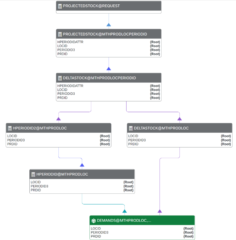
The following calculation graph shows each calculation step in the calculation chain.
190
PUBLIC
Model Conguration Guide
Key Figure Calculations


11.11.2Last Period Aggregation
Use last period aggregation to display the key gure value for the last period in a given time period (for
example, the last month of a quarter or the last month of a year). You can use the IBP_LPA function to
congure last period aggregation in one step.
To use last period aggregation, use the IBP_LPA function in the calculation deniton of key gures in the
Planning Areas app: IBP_LPA("INPUTKFID@INPUTPLEVEL").
Last period aggregation must have exactly one input parameter, which is the key gure to be aggregated. This
key gure must be the same as the input of the calculation denition. The input key gure can be stored and
calculated as well. You cannot use IBP_LPA function without an input key gure as no defualt value is provided.
The result of last period aggregation is written to the output key gure.
Last period aggregation cannot be used in a REQUEST level calculation.
For more information about modeling requirements regarding last period aggregation, see section Checks for
Last Period Aggregation in Key Figures [page 327].
There are two ways to calculate last period aggregation depending on whether a root time prole level is
dened in the output planning level.
Dynamic Aggregation
In case of dynamic last period aggregation, the time prole level for which we aggregate is dened during
runtime. This means that the aggregated key gure can be calculated on any time prole level. The time
aggregation will happen on the requested time granularity. Use this option when you want to ensure exibility
at querying key gures at request level.
To calculate dynamic aggregation, use the IBP_LPA function, and make sure that no root time prole level
is dened in the output planning level of the aggregation and in any of the calculations built on last period
aggregation. Additionally, time prole levels must be the same in the input and output planning levels.
Example
In this example, the input key gure shows the inventory level of a product on a daily basis. We use the
IBP_LPA function to calculate the aggregated inventory level; however, we do not dene the time granularity at
this point. The time prole level for which aggregation takes place is dened during runtime.
AGGRINVENTORY@PERPRODLOC = IBP_LPA("INVENTORY@DAYPRODLOC")
AGGRINVENTORY@REQUEST = SUM("AGGRINVENTORY@PERPRODLOC")
192
PUBLIC
Model Conguration Guide
Key Figure Calculations

Static Aggregation
In case of static last period aggregation, aggregation is dened for a specic time prole level. To calculate
static aggregation, use the
IBP_LPA function and dene a root time prole level in the output planning level.
The root time
prole level in the output planning level must be a possible parent of the root time prole level in
the input planning level.
Note
Static last period aggregation imposes lter blocks in the calculation graph of a key gure, which might
increase the runtime of queries. For more information, see Filter Blocks [page 482].
Example
In this example, the input key gure shows the inventory level of a product on a daily basis. First, we use the
IBP_LPA fuction to calculate the aggregated inventory level on a weekly basis (technical week), as all the other
calculations built on this key gure are dened for calendar and technical weeks. Then, on REQUEST level, we
can calculate the aggregated inventory for all time prole levels that are built on technical week, for example,
calendar week. In this case, aggregation to a higher time prole level will use the REQUEST level aggregation
instead of last period aggregation.
AGGRINVENTORY@TECHWKPRODLOC = IBP_LPA("INVENTORY@DAYPRODLOC")
AGGINVENTORY@REQUEST = SUM("AGGINVENTORY@TECHWKPRODLOC")
Missing Inputs
The last period aggregation function does not generate missing time periods and key gure data in case the
uploaded data is fragmented or missing. The input key gure has to have data uploaded for the last time
period. If there is no data available for the last period or for the entire time horizon, last period aggregation
returns no value.
Last period aggregation uses the time prole of the planning area to nd out the related time periods. The
IBP_LPA function works based on calendar only, it does not consider product combinations at data upload. It
means that if a product has no uploaded data for the requested last period, the function will return no value
and product either. It is the responsibility of the modeling expert to take care of key gure initialization or
defualting when uploading and importing key gures.
Example: Missing key gure in the last period
In this example, there is no data uploaded for the last period (06.01.2019) in the given time period, so the
IBP_LPA function returns no value.
Model Conguration Guide
Key Figure Calculations
PUBLIC 193

Example: Missing key gure in product combination
In this example, there is no uploaded data for Product B and Product C for all time periods, so the IBP_LPA
function returns value for Product A only.
The result of last period aggregation:
Aggregation and Disaggregation Rules
The same aggregation and disaggregation rules apply for last period aggregation as for any other type of
aggregation, as described in section Checks for the Aggregation and Disaggregation Mode in Planning Areas
[page 322].
Last period aggregation is a time-based aggregation. From the available options, disaggregation mode Copy
Value and proportionality No Proportional Disaggregation and Same Key Figure - Stored Values return correct
values after editing a key gure that was calculated using last period aggregation.
Example: Last period aggregation combined with Copy Value and No Proportional
Disaggregation
194
PUBLIC
Model Conguration Guide
Key Figure Calculations

Example: Last period aggregation combined with Copy Value and Same Key Figure - Stored
Values
Note
You cannot use the IBP_LPA function at the base planning level in the calculation graph of a key gure that
is used as the input of a supply planning or forecast consumption operator.
You have the following option, if you want to use the IBP_LPA function in the calculation graph of these
operators:
• Copy the result of the IBP_LPA function to another key gure and use it as the input of the supply
planning or forecast consumption operator.
You cannot use the IBP_LPA function at the base planning level in the calculation graph of a key gure that
uses the output of a supply planning or forecast consumption operator.
You have the following options, if you want to use the output of these operators in the calculation graph of
such key gures:
• Use the IBP_LPA function in calculations at planning levels other than the base planning level of the
key gure in question.
• Copy the result of the IBP_LPA function to another key gure and add the output of the supply
planning or forecast consumption operator as an input of the key gure.
For more information, see section Additional Checks for a Planning Area Enabled for Time-Series-Based
Supply Planning in Planning Areas [page 322].
Related Information
Planning Areas [page 322]
Model Conguration Guide
Key Figure Calculations
PUBLIC 195

11.11.3Rolling Aggregation
Use rolling aggregation to aggregate key gures across several time periods, for a specied time window.
Instead of requesting an L script to create such an aggregation, you can use the IBP_RAGGR function to
congure rolling aggregation in one step.
To use rolling aggregation, use the IBP_RAGGR function in the calculation denition of key gures in the
Planning Areas app. The parameters you dene in the calculation denition specify the time window and the
aggregation type of the rolling aggregation function.
Note
Rolling aggregation imposes lter blocks in the calculation graph of a key gure, which might increase the
runtime of queries. For more information, see Filter Blocks [page 482].
Example
AGGREGATEDDEMAND@PERPRODLOC = IBP_RAGGR ("DEMAND@PERPRODLOC", ''SUM'', -1, 3,
''PASTCURRENTFUTURE'')
In this example, you can calculate the summary of the demand for the previous, actual, and upcoming months.
Parameters of the Rolling Aggregation (IBP_RAGGR) Function
The IBP_RAGGR function has ve mandatory parameters and one optional parameter.
Note
The value of the 1st parameter must be surrounded by double quotation marks.
The values of the 2nd and 5th parameters must be surrounded by two pairs of single quotation marks. A
double quotation mark instead of two single quotation mark will result in an error during activation.
• 1st parameter: input key gure at input planning level (mandatory)
The rst parameter of the IBP_RAGGR function is always the input key gure at the input planning level; for
example, "DEMAND@PERPRODLOC".
• 2nd parameter: aggregation type (mandatory)
The second parameter denes how the key gure is going to be aggregated over the time periods specied
by the third and fourth parameters.
Possible values are MIN, MAX, SUM, AVG, COUNT, and STDDEV.
196
PUBLIC
Model Conguration Guide
Key Figure Calculations
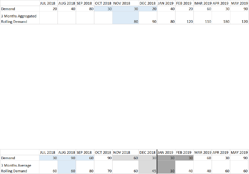
• 3rd parameter: start of rolling aggregation (mandatory)
The third parameter determines the start of the time window for which rolling aggregation is calculated for
the input key gure. It species the starting time period in relation to the actual time period, and it uses the
root time period of the input planning level. It must be an integer.
Possible values:
• Negative integer: rolling aggregation starts before the actual time period
• Zero: rolling aggregation starts with the actual time period
• Positive integer: rolling aggregation starts after the actual time period
For example, if the root time period is month, and the third parameter is -1, aggregation will always start in
the previous month.
• 4th parameter: duration of rolling aggregation (mandatory)
The fourth parameter denes the duration of the rolling aggregation, that is, the number of time periods for
which the input key gure will be aggregated. It has to be a positive integer.
For example, if the root time period is month, the third parameter is -1 and the fourth parameter is 3, the
key gure will be aggregated for the previous, actual, and the upcoming months.
• 5th parameter: calculation horizon (mandatory)
The fth parameter denes the calculation horizon, which can control the output of the calculation. If
separate key gures are used to calculate the past, present, and future values, this parameter lters the
values, thus improves performance in the planning view.
Possible values are PAST, PASTCURRENT, PASTCURRENTFUTURE, CURRENT, CURRENTFUTURE, and FUTURE.
If you use one key gure for rolling aggregation, regardless of the horizon, use the PASTCURRENTFUTURE
value for this parameter.
Example
AGGREGATEDDEMAND@PERPRODLOC = IBP_RAGGR ("DEMAND@PERPRODLOC", ''SUM'', -1, 3,
''CURRENTFUTURE'')
In this example, the value of the calculation horizon is CURRENTFUTURE. This means that
rolling aggregation is only calculated for the current and future time periods, that is, the
AGGREGATEDDEMAND@PERPRODLOC key gure does not have values for time periods before October 2018.
However, values from past time periods are used to calculate the values for current and future time
periods.
• 6th parameter: restart of rolling aggregation (optional)
The last parameter is optional, and it species when rolling aggregation will restart. If you want to restart
aggregation at certain time intervals, enter the time prole level at the end of which aggregation should
stop and restart from 0.
Possible values: All time prole levels that are assigned to the planning level, except for the root time prole
level.
For example, if you enter 6 (year), rolling aggregation will always restart at the rst root time period of the
next year.
Example
AVERAGEDEMAND@PERPRODLOC = IBP_RAGGR ("DEMAND@PERPRODLOC", ''AVG'', -1, 3,
''PASTCURRENTFUTURE'', 6)
Model Conguration Guide
Key Figure Calculations
PUBLIC 197

In this example, you can calculate the average demand for the previous, actual, and upcoming months,
restarting at the rst month of every year.
Modeling Requirements for the Rolling Aggregation (IBP_RAGGR) Function
• A rolling aggregation calculation must have exactly one input.
• The input planning level and the output planning level of a rolling aggregation must be compatible with
each other. That is, they must contain the same set of attributes, including the same set of root attributes.
• Rolling aggregations must be time dependent. That is, both the input planning level and the output
planning level of the calculation must have one of the PERIODID(n) attributes set as the time root
attribute. The time root attribute mustn't be the PERIODID attribute.
The same PERIODID(n) attribute must be the time root attribute in both planning levels.
• The output planning level must have master data type roots.
• The IBP_RAGGR function must have values specied for the 5 mandatory parameters, and can have a value
specied for one optional parameter.
• The rst parameter must be the input key gure at the input planning level.
• The value that is specied for the sixth parameter (time prole level at which the rolling aggregation
restarts) must exist in the time prole assigned to the planning area.
• Only a time prole level that is assigned to the planning level of the rolling aggregation as a time attribute
(but not as a root attribute) can be specied as the value of the sixth parameter of IBP_RAGGR (time
prole level at which the rolling aggregation restarts).
• The IBP_RAGGR function cannot be used at REQUEST level.
• When a calculation graph includes a rolling aggregation, the topmost key gure in the calculation graph
mustn't be editable.
• The IBP_RAGGR function cannot be nested in other calculations.
• To ensure that calculation results are correct, check that there aren’t any NULL values in the root attributes
of the input planning levels.
Note
You cannot use the IBP_RAGGR function at the base planning level in the calculation graph of a key gure
that is used as the input of a supply planning or forecast consumption operator.
You have the following option, if you want to use the IBP_RAGGR function in the calculation graph of these
operators:
• Copy the result of the IBP_RAGGR function to another key gure and use it as the input of the supply
planning or forecast consumption operator.
You cannot use the IBP_RAGGR function at the base planning level in the calculation graph of a key gure
that uses the output of a supply planning or forecast consumption operator.
You have the following options, if you want to use the output of these operators in the calculation graph of
such key gures:
• Use the IBP_RAGGR function in calculations at planning levels other than the base planning level of the
key gure in question.
• Copy the result of the IBP_RAGGR function to another key gure and add the output of the supply
planning or forecast consumption operator as an input of the key gure.
198
PUBLIC
Model Conguration Guide
Key Figure Calculations

For more information, see section Additional Checks for a Planning Area Enabled for Time-Series-Based
Supply Planning in Planning Areas [page 322].
Missing Inputs
You cannot use the IBP_RAGGR function without an input key gure as no default value is provided. The rolling
aggregation function does not generate missing time periods and key gure data in case the uploaded data is
fragmented or missing. The input key gure has to have data uploaded for all time periods. There are two cases
of missing inputs.
Empty Value
If a time period for a planning object combination is missing, that time period is skipped and the value
uploaded to the next time period is taken into account when calculating rolling aggregation. Additionally, rolling
aggregation is not calculated for the missing time period.
NULL Value
If the value of the input key gure is NULL, it is ignored during calculation, but the time window is not extended
with another time period. You can default the NULL value to 0 by adding another calculation if it is justied by
your modeling requirements.
Example
AGGREGATEDDEMAND@PERPRODLOC = IBP_RAGGR ( "DEMAND@PERPRODLOC" , ''AVG'' , -1 , 3,
''PASTCURRENTFUTURE'')
In this example, time period March 2019 is missing. As shown in the table above, March 2019 is skipped and
aggregation continues with the value uploaded to April 2019. That is, instead of calculating the average of
January, February, and March, average is calculated for January, February, and April.
For time period August 2018, the value of the input key gure is NULL. In this case, August 2018 is ignored,
that is, average is calculated for September and October only.
11.11.4Dynamic Rolling Aggregation
Use dynamic rolling aggregation to aggregate key gures across several time periods for a time window
specied by key gures, attributes, or constants. Instead of requesting an L script to create such an
aggregation, you can use the IBP_DYNAMIC_RAGGR function to congure dynamic rolling aggregation in one
step.
With the previous version of Rolling Aggregation [page 196] (IBP_RAGGR), you can dene your calculation
horizon only with constants. Using the dynamic rolling aggregation (IBP_DYNAMIC_RAGGR) function, you have
Model Conguration Guide
Key Figure Calculations
PUBLIC 199

the possibility to dene your calculation horizon with attributes and key gures as well, in addition to constants.
This gives you more exibility in your planning models, but requires more conguration and maintenance
eorts.
Note
Dynamic rolling aggregation imposes lter blocks in the calculation graph of a key gure, which might
increase the runtime of queries. For more information, see Filter Blocks [page 482].
Example
AGGREGATEDDEMAND@PERPRODLOC = IBP_DYNAMIC_RAGGR("DEMAND@PERPRODLOC", ''SUM'',
"AGGROFFSET@PERPRODLOC", "AGGRDURATION@PERPRODLOC", ''PASTCURRENTFUTURE'')
In this example, you can calculate the summary of demand for the time window dened by the
AGGROFFSET@PERPRODLOC and the AGGRDURATION@PERPRODLOC key gures.
Parameters of the Dynamic Rolling Aggregation (IBP_DYNAMIC_RAGGR)
Function
The IBP_DYNAMIC_RAGGR function has ve mandatory parameters and one optional parameter.
Note
Key gure and attribute values must be surrounded by double quotation marks. String constants
(aggregation type and calculation horizon) must be surrended by two pairs of single quotation marks.
Numerical values (for example, restart of rolling aggregation) musn't be surrounded by quotation marks.
• 1st parameter: input key gure at input planning level (mandatory)
The rst parameter of the IBP_DYNAMIC_RAGGR function is always the input key gure to be aggregated at
the input planning level; for example, "DEMAND@PERPRODLOC".
• 2nd parameter: aggregation type (mandatory)
The second parameter denes how the key gure is going to be aggregated over the time periods specied
by the third and fourth parameters.
Possible values are MIN, MAX, SUM, AVG, and COUNT.
• 3rd parameter: start of dynamic rolling aggregation (mandatory)
The third parameter determines the start of the time window for which dynamic rolling aggregation is
calculated for the input key gure. It species the starting time period in relation to the actual time period,
and it uses the root time period of the input planning level.
This parameter can be a constant (integer), an attribute (integer) or a key gure (decimal part is
neglected).
200
PUBLIC
Model Conguration Guide
Key Figure Calculations

Possible values:
• Negative integer: dynamic rolling aggregation starts before the actual time period
• Zero: dynamic rolling aggregation starts with the actual time period
• Positive integer: dynamic rolling aggregation starts after the actual time period
Example: Start of aggregation is dened by an attribute
AGGREGATEDDEMAND@PERPRODLOC = IBP_DYNAMIC_RAGGR("DEMAND@PERPRODLOC", ''SUM'',
"AGGROFFSET", "AGGRDURATION@PERPRODLOC", ''PASTCURRENTFUTURE'')
In this example, for each location/product combination, the start of aggregation is dened by the
AGGROFFSET attribute. For the Boston/Converter combination, the aggregation always starts one month
before (AGGROFFSET=-1), whereas for the Boston/Charger combination, the aggregation always starts
with the actual month (AGGROFFSET=0). The duration is dened by the AGGRDURATION@PERPRODLOC key
gure.
Example: Start of aggregation is dened by a key gure
AGGREGATEDDEMAND@PERPRODLOCCUST = IBP_DYNAMIC_RAGGR("DEMAND@PERPRODLOCCUST",
''SUM'', "AGGROFFSET@PERPRODLOC", "AGGRDURATION@PERPRODLOC",
''PASTCURRENTFUTURE'')
In this example, the start and duration of dynamic rolling aggregation are dened by key gures. If the key
gure value includes decimals, the decimal parts are neglected when calculating the time window of the
aggregation. For example, the value of the AGGROFFSET@PERPRODLOC key gure is -1.1 for August 2020,
which means that aggregation will start with previous month for this period.
Note
If you want a dierent rounding method, use one of the available rounding functions (for example,
ROUND, FLOOR, or CEIL. For more information, see Commonly Used Functions and Expressions [page
162].
• 4th parameter: duration of dynamic rolling aggregation (mandatory)
The fourth parameter denes the duration of the dynamic rolling aggregation, that is, the number of time
periods for which the input key gure will be aggregated.
This parameter can be a constant (integer), an attribute (integer) or a key gure (decimal part is
neglected).
Its value has to be a positive integer. If the value is negative or zero, the result of the dynamic rolling
aggregation will be NULL for the given time period.
Example: Duration of aggregation is dened by an attribute
AGGREGATEDDEMAND@PERPRODLOC = IBP_DYNAMIC_RAGGR("DEMAND@PERPRODLOC", ''SUM'',
"AGGROFFSET", "AGGRDURATION", ''PASTCURRENTFUTURE'')
Model Conguration Guide
Key Figure Calculations
PUBLIC 201

In this example, the start and duration of the dynamic rolling aggregation are dened by attributes for each
location/product combination. For the Boston/Converter combination, the aggregation always starts one
month before (AGGROFFSET=-1) and lasts for 3 months (AGGRDURATION=3). Whereas, for the Boston/
Charger combination, the aggregation always starts with the actual month (AGGROFFSET=0) lasts for 2
months (
AGGRDURATION=2).
Example: Duration of aggregation is dened by a key gure
AGGREGATEDDEMAND@PERPRODLOC = IBP_DYNAMIC_RAGGR("DEMAND@PERPRODLOC", ''SUM'', 0,
"AGGRDURATION@PERPRODLOC", ''PASTCURRENTFUTURE'')
In this example, the start of the aggregation is dened by a constant (0) and the duration is dened by the
AGGRDURATION@PERPRODLOC key gure.
Example: Duration of aggregation is negative or zero
AGGREGATEDDEMAND@PERPRODLOC = IBP_DYNAMIC_RAGGR("DEMAND@PERPRODLOC", ''SUM'',
"AGGROFFSET@PERPRODLOC", "AGGRDURATION@PERPRODLOC", ''PASTCURRENTFUTURE'')
In this example, the duration of the aggregation is negative in September 2020 and zero in April 2021. As a
result, the AGGREGATEDDEMAND key gure is NULL for both periods. If the start or duration of aggregation
is NULL, the output of the IBP_DYNAMIC_RAGGR function is NULL as well, as it is the case for November
2020.
• 5th parameter: calculation horizon (mandatory)
The fth parameter denes the calculation horizon, which can control the output of the calculation. If
separate key gures are used to calculate the past, present, and future values, this parameter lters the
values, thus improves performance in the planning view.
Possible values are PAST, PASTCURRENT, PASTCURRENTFUTURE, CURRENT, CURRENTFUTURE, and FUTURE.
If you use one key gure for dynamic rolling aggregation, regardless of the horizon, use the
PASTCURRENTFUTURE value for this parameter.
Example: Calculation horizon is CURRENTFUTURE
AGGREGATEDDEMAND@PERPRODLOC = IBP_DYNAMIC_RAGGR("DEMAND@PERPRODLOC", ''SUM'',
"AGGROFFSET@PERPRODLOC", "AGGRDURATION@PERPRODLOC", ''CURRENTFUTURE'')
In this example, the value of the calculation horizon is CURRENTFUTURE. This means that dynamic
rolling aggregation is only calculated for the current (February 2021) and future time periods, that is,
the AGGREGATEDDEMAND@PERPRODLOC key gure does not have values for time periods before February
2021. However, values from past time periods are used to calculate the values for current and future time
periods.
• 6th parameter: restart of dynamic rolling aggregation (optional)
The last parameter is optional, and it species when dynamic rolling aggregation will restart. If you want
to restart aggregation at certain time intervals, enter the time prole level at the end of which aggregation
should stop and restart from 0.
202
PUBLIC
Model Conguration Guide
Key Figure Calculations

Possible values: All time prole levels that are assigned to the planning level, except for the root time prole
level.
For example, if you enter 6 (year), dynamic rolling aggregation will always restart at the rst root time
period of the next year.
Example: Restarting aggregation at the rst month of every year
AGGREGATEDDEMAND@PERPRODLOC = IBP_DYNAMIC_RAGGR("DEMAND@PERPRODLOC", ''AVG'',
"AGGROFFSET@PERPRODLOC", "AGGRDURATION@PERPRODLOC", ''PASTCURRENTFUTURE'', 6)
In this example, you can calculate the average demand for the previous, actual, and upcoming months,
restarting at the rst month of every year.
Modeling Requirements for the Dynamic Rolling Aggregation
(IBP_DYNAMIC_RAGGR) Function
• A dynamic rolling aggregation must have one, two, or three input key gures, which must be used in the
calculation expression as well. The rst one is the input key gure to be aggregated, the second one (if
used) denes the start of aggregation, and the third one (if used) denes the duration of the aggregation.
• The attributes of the output planning level must be the union of the attributes of the input planning levels.
• Maximum two input planning levels are allowed.
• Dynamic rolling aggregations must be time dependent. That is, both the input planning levels and the
output planning level of the calculation must have one of the PERIODID(n) attributes set as the time root
attribute. The time root attribute mustn't be the PERIODID attribute.
The same PERIODID(n) attribute must be the time root attribute in both planning levels.
• The output planning level must have master data type roots.
• The IBP_DYNAMIC_RAGGR function must have values specied for the 5 mandatory parameters, and can
have a value specied for one optional parameter.
• The rst parameter must be the input key gure to be aggregated at the input planning level.
• The value that is specied for the sixth parameter (time prole level at which the dynamic rolling
aggregation restarts) must exist in the time prole assigned to the planning area.
• Only a time prole level that is assigned to the planning level of the dynamic rolling aggregation as
a time attribute (but not as a root attribute) can be specied as the value of the sixth parameter of
IBP_DYNAMIC_RAGGR (time prole level at which the dynamic rolling aggregation restarts).
• The IBP_DYNAMIC_RAGGR function cannot be used at REQUEST level.
• When a calculation graph includes a dynamic rolling aggregation, the topmost key gure in the calculation
graph mustn't be editable.
• The IBP_DYNAMIC_RAGGR function cannot be nested in other calculations.
Note
You cannot use the IBP_DYNAMIC_RAGGR function at the base planning level in the calculation graph of a
key gure that is used as the input of a supply planning or forecast consumption operator.
Model Conguration Guide
Key Figure Calculations
PUBLIC 203

You have the following option, if you want to use the IBP_DYNAMIC_RAGGR function in the calculation graph
of these operators:
• Copy the result of the IBP_DYNAMIC_RAGGR function to another key gure and use it as the input of
the supply planning or forecast consumption operator.
You cannot use the IBP_DYNAMIC_RAGGR function at the base planning level in the calculation graph of a
key gure that uses the output of a supply planning or forecast consumption operator.
You have the following options, if you want to use the output of these operators in the calculation graph of
such key gures:
• Use the IBP_DYNAMIC_RAGGR function in calculations at planning levels other than the base planning
level of the key gure in question.
• Copy the result of the IBP_DYNAMIC_RAGGR function to another key gure and add the output of the
supply planning or forecast consumption operator as an input of the key gure.
For more information, see section Additional Checks for a Planning Area Enabled for Time-Series-Based
Supply Planning in Planning Areas [page 322].
Missing Inputs
You cannot use the IBP_DYANAMIC_RAGGR function without an input key gure as no default value is provided.
The dynamic rolling aggregation function does not generate missing time periods and key gure data in case
the uploaded data is fragmented or missing. The input key gures have to have data uploaded for all time
periods. There are two cases of missing inputs.
NULL Value
If the value of the input key gure is NULL, it is ignored during calculation, but the time window is not extended
with another time period. You can default the NULL value to 0 by adding another calculation if it is justied by
your modeling requirements.
Empty Value
If a time period for a planning object combination is missing, it is handled as if the value of the input key gure
were NULL. It is ignored during calculation, but the time window is not extended with another time period. This
is a dierence compared to the IBP_RAGGR function, where the time window is extended.
Example: Missing inputs with SUM
AGGREGATEDDEMAND@PERPRODLOC = IBP_DYNAMIC_RAGGR("DEMAND@PERPRODLOC", ''SUM'',
"AGGROFFSET@PERPRODLOC", "AGGRDURATION@PERPRODLOC", ''PASTCURRENTFUTURE'')
In this example, the value of the input key gure is NULL for November 2020 and December 2020. As a
result, aggregated demand is not calculated for November 2020, the value of the output key gure is NULL.
In addition to that, time periods March 2021 and April 2021 are missing. When calculating dynamic rolling
204
PUBLIC
Model Conguration Guide
Key Figure Calculations

aggregation, the values of the input key gure for these periods are treated as if they were NULL. Again, this
means that the output key gure is NULL for February 2021.
Example: Missing inputs with COUNT
AGGREGATEDDEMAND@PERPRODLOC = IBP_DYNAMIC_RAGGR("DEMAND@PERPRODLOC", ''COUNT'',
"AGGROFFSET@PERPRODLOC", "AGGRDURATION@PERPRODLOC", ''PASTCURRENTFUTURE'')
In these examples, values are aggregated with COUNT. In the case of NULL and missing input key gure values,
the value of the output key gure is 0.
Example: Start and duration of aggregation is NULL
AGGREGATEDDEMAND@PERPRODLOC = IBP_DYNAMIC_RAGGR("DEMAND@PERPRODLOC", ''SUM'',
"AGGROFFSET@PERPRODLOC", "AGGRDURATION@PERPRODLOC", ''PASTCURRENTFUTURE'')
If the start or duration of aggregation is NULL, the output of the IBP_DYNAMIC_RAGGR function is NULL as
well. In this example, both the start and duration of aggregation is NULL for November 2020. As a result, the
value of the output key gure is NULL.
11.11.5Period Shift
Use period shift to shift key gure values by time periods. Instead of using complicated attribute
transformations, you can use the IBP_PERIODSHIFT function to congure period shift in one step.
To use period shift, use the IBP_PERIODSHIFT function in the calculation denition of key
gures in the Planning Areas app: IBP_PERIODSHIFT(<KEY FIGURE@PLANLEVEL>,<NUMBER OF
PERIODS>,<AGGREGATION TYPE>).
Note
Period shift imposes lter blocks in the calculation graph of a key gure, which might increase the runtime
of queries. For more information, see Filter Blocks [page 482].
Model Conguration Guide
Key Figure Calculations
PUBLIC 205

Parameters of the Period Shift (IBP_PERIODSHIFT) Function
The
IBP_PERIODSHIFT function has two mandatory parameters and one optional parameter:
• 1st parameter: input key gure at input planning level (mandatory)
The rst parameter of the IBP_PERIODSHIFT function is always the input key gure at the input planning
level; for example, "ACTUALSQTY@MTHPRODLOC". Period shift is based on the root time attribute of the
planning level of the input key gure.
The value must be surrounded by double quotation marks.
• 2nd parameter: number of periods by which you want to shift the input key gure (mandatory)
You can specify the number of periods the following ways:
• Dene the exact number of time periods, that is, use a constant.
• Use an attribute, which is not a time prole attribute, to dene the number of time periods.
• Use an attribute, which is a time prole attribute, to dene the number of time periods.
• Use a key gure to specify the number of time periods.
If you use an attribute or key gure to specify the number of periods, the value must be surrounded by
double quotation marks.
Conguration
Flexibility Maintenance
Shift by a Constant * * *
Shift by an Attribute * ** **
Shift by a Time Prole At
tribute
** ** **
Shift by a Key Figure *** *** ***
• 3rd parameter: aggregation type (optional)
The third parameter denes how the key gure value is going to be aggregated if the calculation uses
values from more than one time period. If you shift a key gure by a time prole attribute or a key gure,
you might end up with multiple values in some of the time buckets. In this case, you must use the third
parameter or create an aggregation calculation on top of the IBP_PERIODSHIFT function to dene how
the key gure value is calculated from the multiple values of the given time buckets.
Possible values are MIN, MAX, SUM and AVG.
The value must be surrounded by two pairs of single quotation marks. A double quotation mark instead of
two single quotation mark will result in an error during activation.
Shift by a Constant
Use a constant to dene the number of periods by which you want to shift the input key gure. The number has
to be either a positive integer (you shift into the future) or a negative integer (you shift into the past). If you shift
a key gure by a constant, you do not need to dene the third parameter or create an aggregation calculation
on top of the IBP_PERIODSHIFT function.
Example
ACTUALSQTYOFFSET@REQUEST = SUM("ACTUALSQTYOFFSET@MTHPRODLOC")
206
PUBLIC
Model Conguration Guide
Key Figure Calculations

ACTUALSQTYOFFSET@MTHPRODLOC = IBP_PERIODSHIFT("ACTUALSQTY@MTHPRODLOC", 12)
In this example, you can shift the value of actual quantity by 12 months in to the future.
Shift by an Attribute
Attribute Is Not a Time Prole Attribute
Use an attribute, which is not a time prole attribute, to dene the number of periods by which you want to
shift the input key gure. The type of the attribute has to be integer. In this case, the attribute is not assigned
to the time prole; it is assigned to a master data type. If you shift a key gure by an attribute that is not a time
prole attribute, you do not need to dene the third parameter or create an aggregation calculation on top of
the IBP_PERIODSHIFT function.
Example
ACTUALSQTYOFFSET@REQUEST = SUM("ACTUALSQTYOFFSET@MTHPRODLOC")
ACTUALSQTYOFFSET@MTHPRODLOC = IBP_PERIODSHIFT("ACTUALSQTY@MTHPRODLOC", "LEADTIME")
LEADTIME is an attribute to indicate lead times for supply planning for shifting key gures. Dierent products
can have dierent lead times in terms of shipping depending on the product characteristics (for example, size
and weight). In this example, the value of LEADTIME is 1 for PRDID1, and 2 for PRDID2. That is, you shift the
value of actual quantity by 1 in case of product 1, and by 2 in case of product 2.
Attribute Is a Time Prole Attribute
Use a time prole attribute to dene the number of periods by which you want to shift the input key gure. In
this case, the attribute is assigned to the time prole for each period. If you shift a key gure by a time prole
attribute, you might end up with multiple values in some of the time buckets. In this case, you must use the
third parameter or create an aggregation calculation on top of the IBP_PERIODSHIFT function to dene how
the key gure value is calculated from the multiple values of the given time buckets.
Example
ACTUALSQTYOFFSET@REQUEST = SUM("ACTUALSQTYOFFSET@MTHPRODLOC")
ACTUALSQTYOFFSET@MTHPRODLOC = IBP_PERIODSHIFT("ACTUALSQTY@MTHPRODLOC", "LAG")
In this example, LAG is a time prole attribute, part of the MTHPRODLOC planning level, and it species the
shipping time of a product from a manufacturer to the distribution center. The value of LAG is 2 in 2019,
whereas 1 in 2020.
Model Conguration Guide
Key Figure Calculations
PUBLIC 207

Shift by a Key Figure
Use a key gure to dene the number of periods by which you want to shift the input key gure. If you shift
a key gure by another key gure, you might end up with mutliple values in some of the time buckets. In this
case, you must use the third parameter or create an aggregation calculation on top of the IBP_PERIODSHIFT
function to dene how the key gure value is calculated from the multiple values of the given time buckets.
The planning level of the output key gure must be a subset of the planning level of the key gure used for
shifting the input key gure.
Example
ACTUALSQTYOFFSET@MTHPRODLOC = IBP_PERIODSHIFT("ACTUALSQTY@MTHPRODLOC",
"LAGDECIMAL@MTHPRODLOC", ''SUM'')
In this example, LAGDECIMAL@MTHPRODLOC is a key gure, and it species the lead time, which is dierent
for dierent time periods and products. As a result, the value of the ACTUALSQTYOFFSET key gure might
be calculated from the values of more than 1 time periods, for example, as in the case of April 2019. For
this reason, the third parameter is also used to dene how the key gure value is calculated from the
multiple values of the given time periods. In this example, the sum of the shifted values will be calculated
for ACTUALSQTYOFFSET because the aggregation type is SUM in the function.
In case of decimals, the default rounding method is used. If you want to use another rounding mode,
implement it in a separate calculation, as described in Commonly Used Functions and Expressions [page
162].
Modeling Requirements for the Period Shift (IBP_PERIODSHIFT) Function
• The rst parameter must be the input key gure at the input planning level.
• A period shift calculation must have exactly one input if you shift by a constant or an attribute.
• A period shift calculation must have exactly two inputs if you shift the input key gure by another key
gure.
• The input planning level and the output planning level of a period shift must be compatible with each other.
That is, they must contain the same set of attributes, including the same set of root attributes.
• Period shift must be time dependent. That is, both the input planning level and the output planning level of
the calculation must have one of the PERIODID(n) attributes set as the time root attribute. The time root
attribute mustn't be the PERIODID attribute.
The same PERIODID(n) attribute must be the time root attribute in both planning levels.
• The IBP_PERIODSHIFT function cannot be used at REQUEST level.
• When a calculation graph includes a period shift, the topmost key gure in the calculation graph mustn't be
editable.
208
PUBLIC
Model Conguration Guide
Key Figure Calculations

• The IBP_PERIODSHIFT function cannot be nested in other calculations.
• Dene the third parameter or create an aggregation calculation on top of the IBP_PERIODSHIFT function,
if you shift the input key gure by a time prole attribute or key gure.
• The IBP_PERIODSHIFT function must have values specied for the 2 mandatory parameters.
Note
You cannot use the IBP_PERIODSHIFT function at the base planning level in the calculation graph of a key
gure that is used as the input of a supply planning or forecast consumption operator.
You have the following option, if you want to use the IBP_PERIODSHIFT function in the calculation graph of
these operators:
• Copy the result of the IBP_PERIODSHIFT function to another key gure and use it as the input of the
supply planning or forecast consumption operator.
You cannot use the IBP_PERIODSHIFT function at the base planning level in the calculation graph of a key
gure that uses the output of a supply planning or forecast consumption operator.
You have the following options, if you want to use the output of these operators in the calculation graph of
such key gures:
• Use the IBP_PERIODSHIFT function in calculations at planning levels other than the base planning
level of the key gure in question.
• Copy the result of the IBP_PERIODSHIFT function to another key gure and add the output of the
supply planning or forecast consumption operator as an input of the key gure.
For more information, see section Additional Checks for a Planning Area Enabled for Time-Series-Based
Supply Planning in Planning Areas [page 322].
Missing Inputs
You cannot use the IBP_PERIODSHIFT function without an input key gure as no default value is provided. The
period shift function does not generate missing time periods and key gure data in case the uploaded data is
fragmented or missing. The input key gure has to have data uploaded for all time periods. If a time period or
a planning object combination is missing, that time period is skipped, and nothing is shifted. If the value of the
input key gure is NULL or 0, it is shifted by the dened time periods.
If the second parameter, that is, the number of time periods, is empty, NULL or 0, the value of the input key
gure is not shifted.
We recommend to upload data for all time periods, otherwise you might face performance issues.
Model Conguration Guide
Key Figure Calculations
PUBLIC 209

11.11.6Weighted Average
Instead of using several complex calculations, use the IBP_WEIGHTEDAVG function to calculate weighted
average for a key gure in one step.
To calculate weighted average, use the IBP_WEIGHTEDAVG function in the calculation denition of key gures
in the Planning Areas app: IBP_WEIGHTEDAVG(<KEY FIGURE@PLANLEVEL>,<KEY FIGURE@PLANLEVEL> or
<ATTRIBUTE>,<TYPE OF NUMERATOR>)
Business Example
In this example, there are four products, all belong to the same product family (Smart TV). These products
are shipped to three dierent markets: Germany, USA and France. The same products have dierent prices
at dierent locations. For each product/location combination, the following data is available: price, forecasted
quantity and forecasted revenue (calculated as price multiplied by forecasted quantity).
We can calculate the simple average price with the formula SUM(Price) / number of dierent product/
location combinations (8); however, we are interested in the weighted average price. The formula to calculate
weighted average price is SUM(Price*Forecasted Qty) / SUM(Forecasted Qty). We can easily perform this
calculation on aggregated product family level with the IBP_WEIGHTEDAVG function using forecasted quantity
as the weighting factor:
WEIGHTEDPRICE@REQUEST=IBP_WEIGHTEDAVG("STOREDPRICE@MTHPRODLOC",
"FORECASTEDQTY@MTHPRODLOC", ''CALCULATEDNUMERATOR'')
Parameters of the Weighted Average (IBP_WEIGHTEDAVG) Function
The IBP_WEIGHTEDAVG function has three mandatory parameters:
• 1st parameter: input key gure at input planning level
The rst parameter of the IBP_WEIGHTEDAVG function is always the input key gure at
the input planning level; for example, STOREDPRICE@MTHPRODLOC. The sum of the rst
210
PUBLIC
Model Conguration Guide
Key Figure Calculations

parameter multiplied by the second parameter is the numerator of the calculation, for example,
SUM("STOREDPRICE@MTHPRODLOC"*"ACTUALSQTY@MTHPRODLOC").
The parameter value must be surrounded by double quotation marks.
• 2nd parameter: input key gure at the input planning level or attribute
The second parameter of the IBP_WEIGHTEDAVG function is the denominator of the calculation. In case a
calculated numerator is used in the function, the value of the second parameter is the denominator and
the weight as well.
It is either an input key gure at the input planning level, for example, ACTUALSQTY@MTHPRODLOC or a
master data type attribute (integer), for example, WEIGHT. If it is a master data type attribute, it must be
assigned to the input planning level of the rst key gure.
The parameter value must be surrounded by double quotation marks.
• 3rd parameter: type of numerator
The third parameter of the IBP_WEIGHTEDAVG function denes whether the numerator is stored or
calculated.
Possible values:
• CALCULATEDNUMERATOR
The numerator is calculated; it is the sum of the rst parameter multiplied by the second parameter.
Example
WEIGHTEDPRICE = SUM(STOREDPRICE*ACTUALSQTY) / SUM(ACTUALSQTY)
• STOREDNUMERATOR
The numerator is not calculated; it is simply the sum of the rst parameter. In this case, the
numerator's value already includes a multiplication by the weight.
Example
WEIGHTEDPRICE = SUM(STOREDREV) / SUM(ACTUALSQTY)
The value must be surrounded by two pairs of single quotation marks. A double quotation mark instead of
two single quotation mark will result in an error during activation.
Example: Weighted Average with Calculated Numerator
In this example, we have two products (PRDID1 and PRDID2) available at three locations. For each product/
location combination, we work with the following key gures: actuals quantity and stored price. Actuals
quantity and stored price are available in SAP IBP as stored or calculated key gures.
We want to calculate the weighted price for locations 1, 2 and 3 using stored price (STOREDPRICE) as the input
for all three locations.
Model Conguration Guide
Key Figure Calculations
PUBLIC 211

We calculate weighted average, using STOREDPRICE as the rst parameter and ACTUALSQTY as the second
parameter in the IBP_WEIGHTEDAVG function. Since we want STOREDPRICE to be multiplied by the weight, the
value of the third parameter must be
CALCULATEDNUMERATOR.
STOREDPRICE@REQUEST = SUM("STOREDPRICE@MTHPRODLOC")
ACTUALSQTY@REQUEST = SUM("ACTUALSQTY@MTHPRODLOC")
WEIGHTEDPRICE@REQUEST=IBP_WEIGHTEDAVG("STOREDPRICE@MTHPRODLOC","ACTUALSQTY@MTHPRO
DLOC",''CALCULATEDNUMERATOR'')
Let's take a look at FEB 2020, for example. For LOCID1, weighted price is calculated as follows: (50*100 +
100*200) / (50+100) = 166.6667
Example: Weighted Average with Stored Numerator
In this example, we have two products (PRDID1 and PRDID2) available at three locations again. For each
product/location combination, we work with the following key gures: actuals quantity and stored revenue.
Both actuals quantity and stored revenue are available in SAP IBP as stored or calculated key gures.
We want to calculate the weighted price for locations 1, 2, and 3 using stored revenue (STOREDREV) as the input
for all three locations.
We calculate weighted average, using STOREDREV as the rst parameter and ACTUALSQTY as the second
parameter in the IBP_WEIGHTEDAVG function. Since the numerator already contains a multiplication
by weight, the value of the third parameter must be STOREDNUMERATOR. This means that in the
IBP_WEIGHTEDAVG function, the numerator is simply the sum of STOREDREV.
STOREDREV@REQUEST = SUM("STOREDREV@MTHPRODLOC")
ACTUALSQTY@REQUEST = SUM("ACTUALSQTY@MTHPRODLOC")
212
PUBLIC
Model Conguration Guide
Key Figure Calculations

WEIGHTEDPRICE@REQUEST=IBP_WEIGHTEDAVG("STOREDREV@MTHPRODLOC","ACTUALSQTY@MTHPRODL
OC",''STOREDNUMERATOR'')
Let's take a look at FEB 2020, for example. For LOCID1, weighted price is calculated as follows:
(5000+20000) / (50+100) = 166.6667
Example: Weighted Average Based on Revenue and Quantity with
Conversions
In this example, we have two products (PRDID1 and PRDID2) available at two customers and two locations.
For each product/customer/location combination we work with the following key gures: actuals quantity and
actuals revenue.
We can calculate the actuals price (weighted average) for customer 1 and customer 2 using the
IBP_WEIGHTEDAVG function:
1. Calculate ACTUALSQTY:
ACTUALSQTY@REQUEST = SUM("ACTUALSQTY@WKPRODLOCCUSTUOMTO")
ACTUALSQTY@WKPRODLOCCUSTUOMTO = "ACTUALSQTY@WKPRODLOCCUST" *
"UOMCONVERSIONFACTOR@PRODUOMTO"
2. Calculate ACTUALSREV:
ACTUALSREV@REQUEST = SUM("ACTUALSREV@WKPRODLOCCUSTCURRCURRTOUOMTO")
ACTUALSREV@WKPRODLOCCUSTCURRCURRTO = "EXCHANGERATE@MTHCURRCURRTO" *
"ACTUALSREV@WKPRODLOCCUSTCURR"
3. Calculate ACTUALSPRICE:
ACTUALSPRICE@REQUEST =
IBP_WEIGHTEDAVG("ACTUALSREV@WKPRODLOCCUSTCURRCURRTO","ACTUALSQTY@WKPRODLOCCUSTUO
MTO", ''STOREDNUMERATOR'')
Model Conguration Guide
Key Figure Calculations
PUBLIC 213

Note
As of the 2008 release, this example is available in the SAPIBP1 sample planning area.
Example: Weighted Average With an Attribute
In this example, we have two products (PRDID1 and PRDID2) available at one location. For both product/
location combinations, the stored price (key gure) and the weight (attribute) are available.
We can calculate weighted price with the IBP_WEIGHTEDAVG function, using the WEIGHT attribute as the
second parameter. The attribute is assigned to the Location master data type, and it is assigned to the
MTHPRODLOC and MTHLOC planning levels.
WEIGHTEDPRICE@REQUEST = SUM("WEIGHTEDPRICE@MTHLOC")
WEIGHTEDPRICE@MTHLOC = IBP_WEIGHTEDAVG("STOREDPRICE@MTHPRODLOC", "WEIGHT",
''CALCULATEDNUMERATOR'')
Let's take a look at JAN 2020, for example. Weighted price is calculated as follows: (80*50 + 70*50) / (50+50)
= 52.5
Modeling Requirements for the Weighted Average (IBP_WEIGHTEDAVG)
Function
• A weighted average calculation must have exactly 3 parameters.
• The rst parameter must be the input key gure at the input planning level.
• The second parameter must be either an input key gure at the input planning level or a master data type
attribute.
• If the second parameter is a master data type attribute (integer), it must be assigned to the input planning
level of the rst key gure.
• The third parameter must be either STOREDNUMERATOR or CALCULATEDNUMERATOR.
• The IBP_WEIGHTEDAVG function cannot be nested in other calculations.
214
PUBLIC
Model Conguration Guide
Key Figure Calculations

• The planning level of the output key gure must be the subset of the union of the input planning levels.
• The root time attributes of the input planning levels must be the same.
• The input planning levels cannot be on REQUEST level.
• If the second parameter of the IBP_WEIGHTEDAVG function is a key gure, the input planning levels must
have at least one common non-time root attribute that is included in the output planning level.
• When a calculation graph includes a weighted average calculation, the topmost key gure in the calculation
graph mustn't be editable.
Note
You cannot use the IBP_WEIGHTEDAVG function at the base planning level in the calculation graph of a key
gure that is used as the input of a supply planning or forecast consumption operator.
You have the following option, if you want to use the IBP_WEIGHTEDAVG function in the calculation graph of
these operators:
• Copy the result of the IBP_WEIGHTEDAVG function to another key gure and use it as the input of the
supply planning or forecast consumption operator.
You cannot use the IBP_WEIGHTEDAVG function at the base planning level in the calculation graph of a key
gure that uses the output of a supply planning or forecast consumption operator.
You have the following options, if you want to use the output of these operators in the calculation graph of
such key gures:
• Use the IBP_WEIGHTEDAVG function in calculations at planning levels other than the base planning
level of the key gure in question.
• Copy the result of the IBP_WEIGHTEDAVG function to another key gure and add the output of the
supply planning or forecast consumption operator as an input of the key gure.
For more information, see section Additional Checks for a Planning Area Enabled for Time-Series-Based
Supply Planning in Planning Areas [page 322].
Note
Similarly to other aggregation functions (SUM, MIN, MAX, AVG and COUNT), the IBP_WEIGHTEDAVG function
does not impose lter blocks for attributes that are dropped with the aggregation and removed from the
planning level. This means that lters can be applied for these attributes before the aggregation, assuming
there is no other lter block in the calculations that are built on the IBP_WEIGHTEDAVG function.
11.11.7Coverage
Use the IBP_COVERAGE function to calculate coverage for a key gure in one step.
To calculate coverage, use the IBP_COVERAGE function in the calculation denition of key gures in the
Planning Areas app.
You can use the IBP_COVERAGE function for a variety of business scenarios. For more examples and
implementation ideas, see Days of Coverage [page 221] and Projected Stock [page 229].
Model Conguration Guide
Key Figure Calculations
PUBLIC 215

Note
The coverage function imposes time lter blocks in the calculation graph of a key gure, which might
increase the runtime of queries. For more information, see Filter Blocks [page 482].
Parameters of the Coverage (IBP_COVERAGE) Function
The IBP_COVERAGE has six mandatory parameters and two optional parameters.
1st parameter: an input key gure at the input planning level or a constant (mandatory)
The rst parameter of the IBP_COVERAGE function is the amount that has to be covered by the second
parameter. It’s either an input key gure at the input planning level or a positive number.
In case it’s a key gure, the parameter value must be surrounded by double quotation marks; otherwise,
quotation marks mustn't surround this parameter value.
2nd parameter: an input key gure at the input planning level (mandatory)
The second parameter of the IBP_COVERAGE function has to cover the amount of the rst parameter. It’s an
input key gure at the input planning level.
The parameter value must be surrounded by double quotation marks.
3rd parameter: an input key gure at the input planning level or a constant (mandatory)
The third parameter of the IBP_COVERAGE function is an input key gure at the input planning level or a
positive number.
When calculating coverage, values of the third parameter are aggregated with a SUM for all time periods where
the second parameter covers the amount of the rst parameter. If the second parameter covers only a fraction
of the amount of the rst parameter for a given time period, the same fraction of the third parameter in the
given time period is included in the aggregation.
In case the third parameter is a key gure, its value must be surrounded by double quotation marks; otherwise,
quotation marks mustn't surround this parameter value. To achieve better performance, we suggest that you
use a constant (a positive number) to dene the third parameter, if possible.
4th parameter: start of coverage (mandatory)
The fourth parameter determines whether coverage calculation starts with the value of the current or next
bucket.
Possible values:
• NEXTBUCKET
If the value of the second key gure refers to the amount at the end of the current bucket, calculate
coverage starting from the next bucket using the NEXTBUCKET parameter.
• CURRENTBUCKET
If the value of the second key gure refers to the amount at the beginning of the current bucket, calculate
coverage starting from the current bucket using the CURRENTBUCKET parameter.
216
PUBLIC
Model Conguration Guide
Key Figure Calculations
The value must be surrounded by two pairs of single quotation marks. Using a double quotation mark instead
of two single quotation marks results in an error during activation.
5th parameter: zero coverage (mandatory)
With the fth parameter, you can dene whether the zero value of the second parameter can cover the zero
value of the rst parameter in your coverage calculation.
Possible values:
• USEZEROSTOCK
If you want the zero value of the second parameter to cover the zero value of the rst parameter in your
coverage calculation, enter USEZEROSTOCK.
• IGNOREZEROSTOCK
If you don’t want the zero value of the second parameter to cover the zero value of the rst parameter in
your coverage calculation, enter IGNOREZEROSTOCK.
The value must be surrounded by two pairs of single quotation marks. A double quotation mark instead of two
single quotation marks results in an error during activation.
6th parameter: calculation horizon (mandatory)
The sixth parameter denes the calculation horizon. If separate key gures are used to calculate the past,
present, and future values, this parameter lters the values; thus, coverage is only calculated for the specied
time horizon.
Possible values are PAST, PASTCURRENT, PASTCURRENTFUTURE, CURRENT, CURRENTFUTURE, and FUTURE.
However, if you want to see the results of your calculation at REQUEST level, the only possible value is
PASTCURRENTFUTURE.
If you use one key gure for coverage, regardless of the horizon, use the PASTCURRENTFUTURE value for this
parameter.
The value must be surrounded by two pairs of single quotation marks. A double quotation mark instead of two
single quotation marks results in an error during activation.
7th parameter: innite coverage (optional)
The seventh parameter, previously called as full horizon covered, is optional. You can use it to notify the planner
that the value of the second parameter for a time period is larger than the sum of the values of the rst key
gure in all the subsequent periods in the planning horizon.
It has to be an integer, possibly a high enough number (for example, 999), to indicate that there is missing
amount of the rst parameter or excessive amount of the second parameter.
If the parameter isn’t dened and the value of the second parameter for a time period is larger than the sum
of the values of the rst key gure, the sum of the values of the third parameter for the remaining future time
periods is displayed as the coverage.
Quotation marks mustn't surround this parameter value.
8th parameter: number of time periods (optional)
The eighth parameter is optional, and you can only use it if you’ve dened the innite coverage parameter as
well. You can use the eighth parameter to dene and thus limit the time window (by specifying the number of
time periods) across which coverage is calculated for a given projected stock value.
Model Conguration Guide
Key Figure Calculations
PUBLIC 217

If you dene the seventh and eighth parameters, the values of demand are included only from the time window
specied by the eighth parameter and not from the entire planning horizon. The value must be a positive
integer between 10 and 183, allowing you to limit the time window in up to half a year in case of daily time
periods.
Quotation marks mustn't surround this parameter value.
Example
DAYSOFSUPPLY@PERPRODLOC = IBP_COVERAGE("DEMAND@PERPRODLOC",
"PROJECTEDSTOCK@PERPRODLOC", 1, ' 'NEXTBUCKET' ', ' 'USEZEROSTOCK' ',
' 'PASTCURRENTFUTURE' ')
In this example, we calculate days of coverage. On June 3, the projected stock (500) can cover the demand for
2 days, June 4 (300) and June 5 (200).
Modeling Requirements for the Coverage (IBP_COVERAGE) Function
• The coverage calculation has 6 mandatory parameters and two optional parameters.
• The IBP_COVERAGE function must have 1, 2 or 3 input key gures.
• The rst parameter must be an input key gure or a positive number.
• The second parameter must be an input key gure.
• The third parameter must be an input key gure or a positive number.
• The input planning levels must be the same.
• The input planning levels and the output planning level of a coverage calculation must have an identical
structure. That is, they must contain the same set of attributes, including the same set of root attributes.
• Unless calculated at REQUEST level, coverage calculations must be time-dependent. That is, both the
input planning level and the output planning level of the calculation must have one of the PERIODID(n)
attributes set as the time root attribute. The time root attribute mustn't be the PERIODID attribute.
The same PERIODID(n) attribute must be the time root attribute in both planning levels, except in
REQUEST level calculations.
• Unless coverage is calculated at REQUEST level, the output planning level must have master data type
roots.
• REQUEST level calculations must have REQUEST level input calculations.
• The IBP_COVERAGE function can't be nested in other calculations.
• When a calculation graph includes a coverage calculation, the topmost key gure in the calculation graph
mustn't be editable.
218
PUBLIC
Model Conguration Guide
Key Figure Calculations

Note
You can't use the IBP_COVERAGE function at the base planning level in the calculation graph of a key gure
that is used as the input of a supply planning or forecast consumption operator.
If you want to use the IBP_COVERAGE function in the calculation graph of these operators, you have the
following option:
• Copy the result of the IBP_COVERAGE function to another key gure and use it as the input of the
supply planning or forecast consumption operator.
You can't use the IBP_COVERAGE function at the base planning level in the calculation graph of a key gure
that uses the output of a supply planning or forecast consumption operator.
You have the following options, if you want to use the output of these operators in the calculation graph of
such key gures:
• Use the IBP_COVERAGE function in calculations at planning levels other than the base planning level of
the key gure in question.
• Copy the result of the IBP_COVERAGE function to another key gure and add the output of the supply
planning or forecast consumption operator as an input of the key gure.
For more information, see section Additional Checks for a Planning Area Enabled for Time-Series-Based
Supply Planning in Planning Areas [page 322].
Missing Inputs
You cannot use the IBP_COVERAGE function without input key gures as no default values are provided. The
coverage function doesn’t generate missing time periods and key gure data in case the uploaded data is
fragmented or missing. The input key gures have to have data uploaded for all the time periods. There are two
cases of missing inputs: empty value and NULL value.
Empty Value
If a time period for a planning object combination is missing, that time period is skipped and the value
uploaded to the next time period is taken into account when calculating coverage. Coverage is not calculated
for the missing time period.
NULL Value
NULL value is handled in the following way:
• If the value of the 1st parameter is NULL, it is considered zero.
• If the value of the 2nd parameter is NULL, the output of the IBP_COVERAGE function will be NULL as well.
• If the value of the 3rd parameter is NULL, it is considered zero.
You can default the NULL value to 0 by adding another calculation if it’s justied by your modeling
requirements.
Model Conguration Guide
Key Figure Calculations
PUBLIC 219

Zero or Negative Values
Zero and negative values are handled in the following way:
• If the value of the 1st parameter is zero or negative, it’s considered zero.
• If the value of the 2nd parameter is zero or negative, the output of the IBP_COVERAGE function will be zero
as well.
• If the value of the 3rd parameter is zero or negative, it’s considered zero.
The handling of zero values depends on the value of the 5th parameter (zero coverage), as discussed
previously. For more information, see the description of the 5th parameter.
Coverage Calculated at Request Level
You can calculate coverage at REQUEST level.
Example
In REQUEST level calculations, the inputs of the coverage calculation are aggregated rst, then the coverage
calculation is executed.
In this example, the projected stock is 500 for LOCID10 and 200 for LOCID20. In the request level calculation,
their aggregation, in this case their SUM, is calculated rst, and then coverage is calculated.
220
PUBLIC
Model Conguration Guide
Key Figure Calculations

Related Information
Days of Coverage [page 221]
Projected Stock [page 229]
11.11.7.1Days of Coverage
In this sample implementation, we use the IBP_COVERAGE function to calculate days of coverage using
demand and projected stock as input key gures.
Using the IBP_COVERAGE function, you can calculate how many days, weeks, months etc. the calculated
projected stock will last based on the planned demand. In this section, we explain how to use the parameters of
the function to calculate days of coverage and provide you with specic examples. For a general description of
the IBP_COVERAGE function, including modeling requirements and recommendations about aggregation, see
Coverage [page 215].
Note
Coverage imposes lter blocks in the calculation graph of a key gure, which might increase the runtime of
queries. For more information, see Filter Blocks [page 482].
Example
DAYSOFSUPPLY@PERPRODLOC = IBP_COVERAGE("DEMAND@PERPRODLOC",
"PROJECTEDSTOCK@PERPRODLOC", "WORKDAYS@PERPRODLOC", ''CURRENTBUCKET'',
''USEZEROSTOCK'', ''PASTCURRENTFUTURE'')
In this example, we calculate days of coverage. In June 2020, the projected stock (500) can cover the demand
for 2 months, June 2020 (300) and July 2020 (200).
Parameters of the Coverage (IBP_COVERAGE) Function to Calculate Days of
Coverage
The IBP_COVERAGE function has six mandatory parameters and two optional parameters.
Model Conguration Guide
Key Figure Calculations
PUBLIC 221
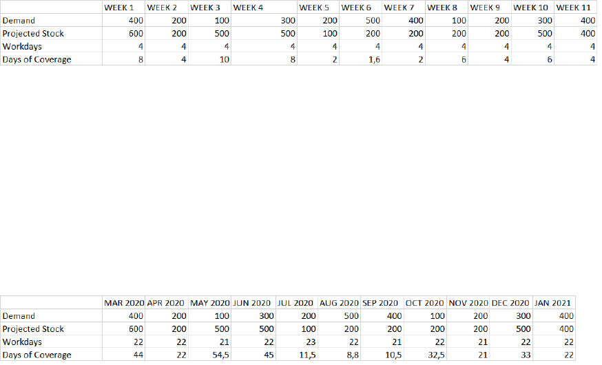
1st parameter: demand (mandatory)
The rst parameter of the IBP_COVERAGE function is the demand. It is either an input key gure at the input
planning level or a positive number. Before performing the coverage calculation, make sure that the demand is
already available at the required planning level. If the value of the key gure is negative, it is counted as zero.
In case it is a key gure, the parameter value must be surrounded by double quotation marks; otherwise,
quotation marks must not surround this parameter value.
2nd parameter: projected stock (mandatory)
The second parameter of the IBP_COVERAGE function is the projected stock (input key gure) at the input
planning level. Before performing the coverage calculation, make sure that the projected stock is already
available at the required planning level. If the value of the key gure is negative, it is counted as zero.
The parameter value must be surrounded by double quotation marks.
3rd parameter: number of working days (mandatory)
The third parameter denes the number of working days for the given time period. First, coverage is calculated
from the demand and projected stock for each period, then the values are multiplied by the number of working
days and summed up.
You have the following options to dene the number of working days:
• Dene the number of working days with a positive number. In this case, we assume that each time period
in your planning horizon is made up of that many working days.
If possible, we suggest that you use a constant (a positive number) to dene the third parameter to achieve
better performance. Quotation marks must not surround this parameter value.
Example
DAYSOFSUPPLY@PERPRODLOC = IBP_COVERAGE("DEMAND@PERPRODLOC" ,
"PROJECTEDSTOCK@PERPRODLOC" , 4 , ''CURRENTBUCKET'', ''USEZEROSTOCK'',
''PASTCURRENTFUTURE'')
In this example, a week always consists of 4 workdays, so for each time period we multiply coverage value
with 4 to calculate the days of coverage.
When no time-based multiplication is required, the value of the parameter must be 1. For example, if
demand and projected stock are on a daily level, and you want to calculate coverage in days as well, enter 1.
• Use a key gure, for example, WORKDAYS@PERPRODLOC, to dene the number of working days for each
time period in your planning horizon. For example, if demand and projected stock are on a monthly level,
you can calculate coverage in days with the help of this key gure.
The parameter value must be surrounded by double quotation marks.
Example
DAYSOFSUPPLY@PERPRODLOC = IBP_COVERAGE("DEMAND@PERPRODLOC" ,
"PROJECTEDSTOCK@PERPRODLOC" , "WORKDAYS@PERPRODLOC" , ''CURRENTBUCKET'',
''USEZEROSTOCK'' , ''PASTCURRENTFUTURE'')
222
PUBLIC
Model Conguration Guide
Key Figure Calculations

In this example, demand and projected stock are on a monthly level, but we want to calculate the coverage
in days. To do so, we use a key gure that denes the number of working days for each time period. When
performing the calculation, we multiply the value of coverage with the number of working days for each
time period and then sum up the values. In March 2020, the projected stock (600) can cover the demand
of March 2020 (400) and April 2020 (200). The number of working days is 22 for both periods, so the days
of coverage is 44 (2*22) for March 2020.
If the value of the key gure is negative, it is counted as zero.
Example: Number of Workdays Is Zero
DAYSOFSUPPLY@PERPRODLOC = IBP_COVERAGE("DEMAND@PERPRODLOC" ,
"PROJECTEDSTOCK@PERPRODLOC" , "WORKDAYS@PERPRODLOC" , ''CURRENTBUCKET'',
''USEZEROSTOCK'' , ''PASTCURRENTFUTURE'')
In this example, the number of workdays is zero on week 4. When calculating the days of coverage for week
3, the projected stock of week 3 can cover the demand of weeks 3, 4, and 5. However, since week 4 has no
workdays, the days of coverage for week 3 is the sum of workdays of weeks 3 and 5.
4th parameter: start of coverage (mandatory)
The fourth parameter determines whether coverage calculation starts with the demand value of the current or
next bucket.
Possible values:
• NEXTBUCKET
If the value of the projected stock key gure refers to the stock at the end of the day, calculate coverage
starting from the next bucket using the NEXTBUCKET parameter.
Example
DAYSOFSUPPLY@PERPRODLOC = IBP_COVERAGE("DEMAND@PERPRODLOC",
"PROJECTEDSTOCK@PERPRODLOC", "WORKDAYS@PERPRODLOC", ''NEXTBUCKET'',
''USEZEROSTOCK'', ''PASTCURRENTFUTURE'')
• CURRENTBUCKET
If the value of the projected stock key gure refers to the stock at the beginning of the day, calculate
coverage starting from the current bucket using the CURRENTBUCKET parameter.
Example
DAYSOFSUPPLY@PERPRODLOC = IBP_COVERAGE("DEMAND@PERPRODLOC",
"PROJECTEDSTOCK@PERPRODLOC", "WORKDAYS@PERPRODLOC", ''CURRENTBUCKET'',
''USEZEROSTOCK'', ''PASTCURRENTFUTURE'')
The value must be surrounded by two pairs of single quotation marks. A double quotation mark instead of two
single quotation mark will result in an error during activation.
Model Conguration Guide
Key Figure Calculations
PUBLIC 223

5th parameter: zero coverage (mandatory)
With the fth parameter, you can dene whether zero stock can cover zero demand or not in your coverage
calculation.
The value must be surrounded by two pairs of single quotation marks. A double quotation mark instead of two
single quotation mark will result in an error during activation.
Possible values:
• USEZEROSTOCK
If you want zero stock to cover zero demand in your coverage calculation, enter USEZEROSTOCK. In this
case, when calculating days or weeks of coverage, time periods with zero demand will be included in the
calculation.
Example
DAYSOFSUPPLY@PERPRODLOC = IBP_COVERAGE("DEMAND@PERPRODLOC",
"PROJECTEDSTOCK@PERPRODLOC", 7, ''CURRENTBUCKET'', ''USEZEROSTOCK'',
''PASTCURRENTFUTURE'')
In these examples, zero stock can cover zero demand. In the rst example, though the projected stock on
week 3 is consumed by the demands of weeks 3, 4, and 5; it can still cover the zero demands of weeks 6 to
12. As a result, the days of coverage is 70 for week 3.
In the second example, though the projected stock is zero on week 5, it can cover the demand of weeks 5 to
11.
If you have zero projected stock and zero demand for a given time frame, the days of coverage will equal
the sum of the working days of the given time frame.
• IGNOREZEROSTOCK
If you do not want zero stock to cover zero demand in your coverage calculation, enter IGNOREZEROSTOCK.
In this case, when calculating days or weeks of supply, time periods with zero demand will not be included
in the calculation.
Example
DAYSOFSUPPLY@PERPRODLOC = IBP_COVERAGE("DEMAND@PERPRODLOC",
"PROJECTEDSTOCK@PERPRODLOC", 7, ''CURRENTBUCKET'', ''IGNOREZEROSTOCK'',
''PASTCURRENTFUTURE'')
As opposed to the previous examples, zero stock cannot cover zero demand in these examples. In the rst
example, the projected stock on week 3 is consumed by the demands of weeks 3, 4, and 5; which means
224
PUBLIC
Model Conguration Guide
Key Figure Calculations

that it cannot cover any further demands, not even zero demands. As a result, the days of coverage is 21 for
week 3.
In the second example, both demand and projected stock equal zero for weeks 5 to 11. Since zero projected
stock cannot cover zero demand, days of coverage will be zero as well for these weeks.
If you have zero projected stock and zero demand for a given time period, the days of coverage for that
time period will be zero as well.
6th parameter: calculation horizon (mandatory)
Possible values are PAST, PASTCURRENT, PASTCURRENTFUTURE, CURRENT, CURRENTFUTURE, and FUTURE.
However, if you want to see the results of your calculation at REQUEST level, the only possible value is
PASTCURRENTFUTURE.
If you use one key gure for coverage, regardless of the horizon, use the PASTCURRENTFUTURE value for this
parameter.
The value must be surrounded by two pairs of single quotation marks. A double quotation mark instead of two
single quotation mark will result in an error during activation.
Example
DAYSOFSUPPLY@PERPRODLOC = IBP_COVERAGE("DEMAND@PERPRODLOC",
"PROJECTEDSTOCK@PERPRODLOC", "WORKDAYS@PERPRODLOC", ''CURRENTBUCKET'',
''USEZEROSTOCK'', ''CURRENTFUTURE'')
In this example, days of coverage is only calculated for current and future time periods.
7th parameter: innite coverage (optional)
The seventh parameter, previously called as full horizon covered, is optional. You can use it to notify the planner
that the projected stock of a time period is larger than the sum of the demands in all the subsequent periods in
the planning horizon.
It has to be an integer, possibly a high enough number (for example, 999), to indicate that there is missing
demand or excessive stock.
If the parameter is not dened and the projected stock is larger than the sum of the demands, the number of
the remaining future time periods (or the sum of the working days for the remaining future time periods) is
displayed as the coverage.
Quotation marks must not surround this parameter value.
Example
DAYSOFSUPPLY@PERPRODLOC = IBP_COVERAGE("DEMAND@PERPRODLOC",
"PROJECTEDSTOCK@PERPRODLOC", 7, ''CURRENTBUCKET'', ''USEZEROSTOCK'',
''PASTCURRENTFUTURE'', 999)
Model Conguration Guide
Key Figure Calculations
PUBLIC 225

In both examples, we use the innite coverage parameter to indicate excessive demand or lack of projected
stock. We use 999 to indicate if projected stock is larger than the sum of the demands. In the rst example,
the projected stock on week 3 equals the sum of the demands for the remaining time periods, so the days of
coverage is the sum of the remaining days in the planning horizon. In the second example, the projected stock
on week 3 is larger than the sum of the demands for the remaining time periods, so the value of the days of
coverage is 999 for week 3.
8th parameter: number of time periods (optional)
The eighth parameter is optional, and you can only use it if you have dened the innite coverage parameter as
well. You can use the eighth parameter to dene and thus limit the time window (by specifying the number of
time periods) across which coverage is calculated for a given projected stock value.
If you dene the seventh and eighth parameters, the values of demand are included only from the time window
specied by the eighth parameter and not from the entire planning horizon. The value must be a positive
integer between 10 and 183, allowing you to limit the time window in up to half a year in case of daily time
periods.
Quotation marks must not surround this parameter value.
Example
DAYSOFSUPPLY@PERPRODLOC = IBP_COVERAGE("DEMAND@PERPRODLOC",
"PROJECTEDSTOCK@PERPRODLOC", 7, ''CURRENTBUCKET'', ''USEZEROSTOCK'',
''PASTCURRENTFUTURE'', 999, 10)
In this example, the value of the eighth parameter is 10. It means that when we calculate coverage, the values
of demand are included from 10 periods starting with the current period. Days of coverage is calculated as
follows:
• Week 3: days of coverage is 999 as the projected stock is larger than the sum of demand for the time
window you have dened (10 periods).
• Week 4: days of coverage is 70 as the projected stock can cover the demand for 10 weeks (70 days).
• Weeks 5-12: as we use zero stock, days of coverage is the sum of the working days with zero demand in the
given time window (10 periods).
• Weeks 13 and 14: days of coverage is 0, as 0 projected stock cannot cover the demands (100 and 300).
If we use NEXTBUCKET instead of CURRENTBUCKET, demand values are included from 10 periods as well, but in
this case starting with the next period.
Note
By dening the number of time periods parameter, you can optimize the performance of your queries if you
use the innite coverage parameter as well. In the coverage calculation, the values of demand are included
only from the time window specied by this parameter and not from the entire planning horizon.
226
PUBLIC
Model Conguration Guide
Key Figure Calculations

However, this also means that using the number of time periods parameter might aect the preciseness
of your calculation and your coverage value might be 999 (or the value you have dened by the seventh
parameter) too frequently. For this reason, we suggest that rst you determine how many time periods you
usually work with when calculating coverage. Then, using the eighth parameter, dene a time window that
contains more time periods than you usually use.
For example, if you calculate coverage for 12 months mostly, set the eighth parameter to 24. This way you
will calculate with demand values from the time window you usually work with, and at the same time you
can optimize performance by not including demand values from time periods that you are not interested in.
Missing Inputs
You cannot use the IBP_COVERAGE function without input key gures as no default values are provided. The
coverage function does not generate missing time periods and key gure data in case the uploaded data is
fragmented or missing. The input key gures have to have data uploaded for all time periods. There are two
cases of missing inputs: empty value and NULL value.
Empty Value
If a time period for a planning object combination is missing, that time period is skipped and the value
uploaded to the next time period is taken into account when calculating coverage. Coverage is not calculated
for the missing time period.
Example: Empty Value
DAYSOFSUPPLY@PERPRODLOC = IBP_COVERAGE("DEMAND@PERPRODLOC",
"PROJECTEDSTOCK@PERPRODLOC", 1, ''CURRENTBUCKET'', ''USEZEROSTOCK'',
''PASTCURRENTFUTURE'')
In this example, time period June 9 is missing. As shown in the table above, June 9 is skipped and coverage
calculation continues with the value uploaded to June 10. Consequently, the days of coverage for June 8 is 2.
NULL Value
NULL value is handled in the following way:
• If the value of demand is NULL, it is considered as zero.
• If the value of projected stock is NULL, the value of days or weeks of coverage will be NULL as well.
• If the value of workdays is NULL, it is considered as zero.
You can default the NULL value to 0 by adding another calculation if it is justied by your modeling
requirements.
Example: Demand is NULL
DAYSOFSUPPLY@PERPRODLOC = IBP_COVERAGE("DEMAND@PERPRODLOC",
"PROJECTEDSTOCK@PERPRODLOC", 1, ''CURRENTBUCKET'', ''USEZEROSTOCK'',
''PASTCURRENTFUTURE'', 999)
Model Conguration Guide
Key Figure Calculations
PUBLIC 227

In this example, the value of planned demand is NULL from June 7, that is, planned demand is zero for June 7
and the remaining time periods. As a result, days of coverage is 999 from June 6, as projected stock is larger
than the sum of the demands for the remaining time periods.
Example: Projected Stock is NULL.
DAYSOFSUPPLY@PERPRODLOC = IBP_COVERAGE("DEMAND@PERPRODLOC",
"PROJECTEDSTOCK@PERPRODLOC", 1, ''CURRENTBUCKET'', ''USEZEROSTOCK'',
''PASTCURRENTFUTURE'', 999)
In this example, days of coverage is NULL on June 7 and June 8 because projected stock is NULL on these days
as well. Now, let's take a look at June 5. Projected stock is 600 on June 6, which can cover the demands from
June 6 to June 10 (600=500+NULL+NULL+100+0). As a result, days of coverage is 5 on June 5.
Zero or Negative Values
Zero and negative values are handled in the following way:
• If the value of demand is zero or negative, it is considered as zero.
• If the value of projected stock is zero or negative, the value of days or weeks of coverage will be zero as
well.
• If the value of workdays is zero or negative, it is considered as zero.
The handling of zero demand and zero projected stock depends on the value of the 5th parameter (zero
coverage), as discussed above. For more information, see the description of the 5th parameter above.
Example: Demand is Negative
DAYSOFSUPPLY@PERPRODLOC = IBP_COVERAGE("DEMAND@PERPRODLOC",
"PROJECTEDSTOCK@PERPRODLOC", 1, ''CURRENTBUCKET'', ''USEZEROSTOCK'',
''PASTCURRENTFUTURE'', 999)
Negative demand is counted as zero demand. In this example, the demand is negative on June 1, which is
calculated as zero. The projected stock on June 1 (600) can cover the demand of June 1 (0) and 75% of the
demand for June 2 (600), so days of coverage equals 1.75.
228
PUBLIC
Model Conguration Guide
Key Figure Calculations

11.11.7.2Projected Stock
In this sample implementation, we use the IBP_COVERAGE function to calculate projected stock using days of
supply and demand as input key gures.
Using the IBP_COVERAGE function, you can calculate how much stock is required to cover the demand based
on the days of supply value. In this section, we explain how to use the parameters of the function to calculate
projected stock and provide you with specic examples. For a general description of the IBP_COVERAGE
function, including modeling requirements and recommendations about aggregation, see Coverage [page 215].
Note
Coverage imposes lter blocks in the calculation graph of a key gure, which might increase the runtime of
queries. For more information, see Filter Blocks [page 482].
Example
PROJECTEDSTOCK@PERPRODLOC = IBP_COVERAGE("WORKDAYS@PERPRODLOC" ,
"DAYSOFSUPPLY@PERPRODLOC" , "DEMAND@PERPRODLOC" , ''CURRENTBUCKET'',
''USEZEROSTOCK'' , ''PASTCURRENTFUTURE'')
In this example, we calculate projected stock. In June 2020, we need to cover the demand for 45 days, that is
for June 2020 (22 days) and July 2020 (23 days). This means that the value of the projected stock for June
2020 is going to be 500 (300+200).
Parameters of the Coverage (IBP_COVERAGE) Function to Calculate Projected
Stock
The IBP_COVERAGE function has six mandatory parameters and two optional parameters.
1st parameter: number of working days (mandatory)
The rst parameter denes the number of working days for the given time period.
You have the following options to dene the number of working days:
• Use a key gure, for example WORKDAYS@PERPRODLOC, to dene the number of working days for each time
period in your planning horizon. For example, if demand is on a monthly level, you can calculate projected
stock in days with the help of this key gure.
The parameter value must be surrounded by double quotation marks.
Example
Model Conguration Guide
Key Figure Calculations
PUBLIC 229

PROJECTEDSTOCK@PERPRODLOC = IBP_COVERAGE("WORKDAYS@PERPRODLOC" ,
"DAYSOFSUPPLY@PERPRODLOC" , "DEMAND@PERPRODLOC" , ''CURRENTBUCKET'',
''USEZEROSTOCK'' , ''PASTCURRENTFUTURE'')
In this example, demand is on a monthly level, however, the time period projected stock needs to cover is
given in days. For example, in June 2020, projected stock needs to cover the demand for 45 days. With
the help of the
WORKDAYS@PERPRODLOC key gure, we can calculate that 45 days cover two months, June
2020 (22 days with a demand of 300) and July 2020 (23 days with a demand of 200). This means that the
value of the projected stock for June 2020 is 500 (300+200).
If the value of the key gure is negative, it is counted as zero.
• Dene the number of working days with a positive number. In this case, we assume that each time period
in your planning horizon is made up of that many working days.
Quotation marks must not surround this parameter value.
Example
PROJECTEDSTOCK@PERPRODLOC = IBP_COVERAGE(7, "DAYSOFSUPPLY@PERPRODLOC",
"DEMAND@PERPRODLOC" , ''CURRENTBUCKET'', ''USEZEROSTOCK'',
''PASTCURRENTFUTURE'')
In this example, a week always consists of 7 workdays. On week 1, the days of supply is 14, that is, the
projected stock needs to cover the demand for 14 days (2 weeks). This means that the demand of week 1
(100) and week 2 (300) has to be covered by the projected stock (400).
2nd parameter: days of supply (mandatory)
The second parameter of the IBP_COVERAGE function is the days of supply (input key gure at the input
planning level). Before performing the projected stock calculation, make sure that the days of supply is already
available at the required planning level. If the value of the key gure is negative, it is counted as zero.
The parameter value must be surrounded by double quotation marks.
3rd parameter: demand (mandatory)
The third parameter of the IBP_COVERAGE function is the demand. It is either an input key gure at the input
planning level or a positive number. Before performing the projected stock calculation, make sure that the
demand is already available at the required planning level. If the value of the key gure is negative, it is counted
as zero.
In case it is a key gure, the parameter value must be surrounded by double quotation marks; otherwise,
quotation marks must not surround this parameter value.
4th parameter: start of coverage (mandatory)
The fourth parameter determines whether projected stock calculation starts with the number of working days
value of the current or next bucket.
Possible values:
• NEXTBUCKET
230
PUBLIC
Model Conguration Guide
Key Figure Calculations

If you want to count the number of working days starting with the next bucket, use the NEXTBUCKET
parameter.
Example
PROJECTEDSTOCK@PERPRODLOC = IBP_COVERAGE("WORKDAYS@PERPRODLOC",
"DAYSOFSUPPLY@PERPRODLOC@PERPRODLOC", "DEMAND@PERPRODLOC", ''NEXTBUCKET'',
''IGNOREZEROSTOCK'', ''PASTCURRENTFUTURE'')
• CURRENTBUCKET
If you want to count the number of working days starting with the current bucket, use the CURRENTBUCKET
parameter.
Example
PROJECTEDSTOCK@PERPRODLOC = IBP_COVERAGE("WORKDAYS@PERPRODLOC",
"DAYSOFSUPPLY@PERPRODLOC@PERPRODLOC", "DEMAND@PERPRODLOC", ''CURRENTBUCKET'',
''USEZEROSTOCK'', ''PASTCURRENTFUTURE'')
The value must be surrounded by two pairs of single quotation marks. A double quotation mark instead of two
single quotation mark will result in an error during activation.
5th parameter: zero coverage (mandatory)
With the fth parameter, you can dene whether zero days of supply can cover zero workdays or not in your
coverage calculation.
The value must be surrounded by two pairs of single quotation marks. A double quotation mark instead of two
single quotation mark will result in an error during activation.
Possible values:
• USEZEROSTOCK
If you want zero days of supply to cover zero workdays, enter USEZEROSTOCK. In this case, when
calculating projected stock, time periods with zero working days will be included in the calculation.
Example
PROJECTEDSTOCK@PERPRODLOC = IBP_COVERAGE("WORKDAYS@PERPRODLOC",
"DAYSOFSUPPY@PERPRODLOC", "DEMAND@PERPRODLOC", ''NEXTBUCKET'', ''USEZEROSTOCK'',
''PASTCURRENTFUTURE'')
In this example, when calculating the projected stock for June 1, the demand value for June 4 is included in
the calculation.
• IGNOREZEROSTOCK
If you do not want zero days of supply to cover zero workdays, enter IGNOREZEROSTOCK. In this case, when
calculating projected stock, time periods with zero working days will not be included in the calculation.
Example
Model Conguration Guide
Key Figure Calculations
PUBLIC 231

PROJECTEDSTOCK@PERPRODLOC = IBP_COVERAGE("WORKDAYS@PERPRODLOC",
"DAYSOFSUPPY@PERPRODLOC", "DEMAND@PERPRODLOC", ''NEXTBUCKET'',
''IGNOREZEROSTOCK'', ''PASTCURRENTFUTURE'')
As opposed to the previous example, when calculating the projected stock for June 1, the demand value for
June 4 is not included in the calculation.
6th parameter: calculation horizon (mandatory)
The sixth parameter denes the calculation horizon. If separate key gures are used to calculate the past,
present, and future values, this parameter lters the values; thus, projected stock will only be calculated for the
specied time horizon.
Possible values are PAST, PASTCURRENT, PASTCURRENTFUTURE, CURRENT, CURRENTFUTURE, and FUTURE.
However, if you want to see the results of your calculation at REQUEST level, the only possible value is
PASTCURRENTFUTURE.
If you use one key gure for projected stock, regardless of the horizon, use the PASTCURRENTFUTURE value for
this parameter.
The value must be surrounded by two pairs of single quotation marks. A double quotation mark instead of two
single quotation mark will result in an error during activation.
Example
PROJECTEDSTOCK@PERPRODLOC = IBP_COVERAGE("WORKDAYS@PERPRODLOC",
"DAYSOFSUPPY@PERPRODLOC", "DEMAND@PERPRODLOC", ''CURRENTBUCKET'', ''USEZEROSTOCK'',
''CURRENTFUTURE'')
In this example, days of coverage is only calculated for current and future time periods.
7th parameter: innite coverage (optional)
The seventh parameter, previously called full horizon covered, is optional. If you use the IBP_COVERAGE
function to calculate project stock, it doesn't have a business meaning. We recommend that you do not use this
parameter in this case.
8th parameter: number of time periods (optional)
The eighth parameter is optional, and you can only use it if you have dened the innite coverage parameter as
well. Since the innite coverage parameter is not recommended for calculating projected stock, we suggest that
you do not use the number of time periods parameter either.
232
PUBLIC
Model Conguration Guide
Key Figure Calculations

Using Aggregation
When the second and third input key gures (days/weeks/months of supply and demand) are on dierent
aggregation levels, you can use the rst parameter (number of working days) to dene the number of time
periods at the time prole level of the second parameter (days/weeks/months of supply). For example, if
demand is available at the level of months, but days of supply is calculated in days, you can use the workdays
parameter to count the number of working days in each month.
Example
PROJECTEDSTOCK@PERPRODLOC = IBP_COVERAGE("WORKDAYS@PERPRODLOC",
"DAYSOFSUPPY@PERPRODLOC", "DEMAND@PERPRODLOC", ''CURRENTBUCKET'', ''USEZEROSTOCK'',
''PASTCURRENTFUTURE'')
In this example, we calculate projected stock for the following 9 cases:
Days of supply
Weeks of supply Months of supply
Demand on daily level Value of the rst parameter is
1 or 0.
First parameter denes the
number of workweeks for
each day.
First parameter denes the
number of work months for
each day.
Demand on weekly level First parameter denes the
number of working days for
each week.
Value of the rst parameter is
1 or 0.
First parameter denes the
number of work months for
each week.
Demand on monthly level First parameter denes the
number of working days for
each month.
First parameter denes the
number of workweeks for
each month.
Value of the rst parameter is
1 or 0.
Cases where the time granularity of days/weeks/months of supply is higher than the time granularity of
demand are indicated with pink in the example above. These cases - though mathematically possible - are most
probably not relevant from a business perspective.
Model Conguration Guide
Key Figure Calculations
PUBLIC 233

Missing Inputs
You cannot use the IBP_COVERAGE function without input key gures as no default values are provided. The
coverage function does not generate missing time periods and key gure data in case the uploaded data is
fragmented or missing. The input key
gures have to have data uploaded for all time periods. There are two
cases of missing inputs: empty value and NULL value.
Empty Value
If a time period for a planning object combination is missing, that time period is skipped and the value
uploaded to the next time period is taken into account when calculating projected stock. Projected stock is not
calculated for the missing time period.
Example: Empty Value
PROJECTEDSTOCK@PERPRODLOC = IBP_COVERAGE("WORKDAYS@PERPRODLOC",
"DAYSOFSUPPY@PERPRODLOC", "DEMAND@PERPRODLOC", ''CURRENTBUCKET'', ''USEZEROSTOCK'',
''PASTCURRENTFUTURE'')
In this example, time period July 2020 is missing. As shown in the table above, July 2020 is skipped and
projected stock calculation continues with the value uploaded to August 2020. Consequently, projected stock
is 800 for June 2020.
NULL Value
NULL value is handled in the following way:
• If the value of workdays is NULL, it is considered as zero.
• If the value of days of supply is NULL, the value of the projected stock will be NULL as well.
• If the value of demand is NULL, it is considered as zero.
You can default the NULL value to 0 by adding another calculation if it is justied by your modeling
requirements.
Example: NULL Values
PROJECTEDSTOCK@PERPRODLOC = IBP_COVERAGE("WORKDAYS@PERPRODLOC",
"DAYSOFSUPPY@PERPRODLOC", "DEMAND@PERPRODLOC", ''CURRENTBUCKET'', ''USEZEROSTOCK'',
''PASTCURRENTFUTURE'')
In this example, all three key gures have NULL values:
• In April 2020, the value of workdays is NULL, which is considered as zero. It means that the 43 days of
supply in March 2020 have to cover the demand for the 22 days of March 2020 (400) and the 21 days of
May 2020 (100). As a result, projected stock is 500 for March 2020.
234
PUBLIC
Model Conguration Guide
Key Figure Calculations

• In August 2020, the value of demand is NULL, which is considered as zero. Since days of supply is 8.8
(less than 22), zero demand entails zero projected stock.
• In December 2020, the value of days of supply is NULL; consequently, the value of the projected stock is
NULL as well.
Zero or Negative Values
Zero and negative values are handled in the following way:
• If the value of workdays is zero or negative, it is considered as zero.
• If the value of days of supply is zero or negative, the value of the projected stock will be zero as well.
• If the value of demand is zero or negative, it is considered as zero.
The handling of zero workdays and zero days of supply depends on the value of the 5th parameter (zero
coverage), as discussed above. For more information, see the description of the 5th parameter above.
Example: Zero Values
PROJECTEDSTOCK@PERPRODLOC = IBP_COVERAGE("WORKDAYS@PERPRODLOC",
"DAYSOFSUPPY@PERPRODLOC", "DEMAND@PERPRODLOC", ''CURRENTBUCKET'', ''USEZEROSTOCK'',
''PASTCURRENTFUTURE'')
In this example, all three key gures have zero values:
• In March 2020, the value of demand is zero. As a result, projected stock is 200 (0+200) for March 2020.
• In August 2020, the value of workdays is zero. It means that the 44 days of supply in July 2020 has to
cover the demand for the 23 days of July 2020 (200) and the 21 days of September 2020 (400). As a
result projected stock is 600 for July 2020.
• In November 2020, the value of days of supply is zero; consequently, the value of projected stock is zero
as well.
11.11.8Calendar
Use the calendar function to count with dierent calendars (integrated from SAP ERP) in key gure
calculations.
To use the calendar function, use the IBP_CALENDAR function in the calculation denition of key gures in the
Planning Areas app: IBP_CALENDAR(<KEY FIGURE@PLANLEVEL, <CALENDAR ATTRIBUTE>)
Parameters of the Calendar (IBP_CALENDAR) Function
The IBP_CALENDAR function has two mandatory parameters:
• 1st parameter: input key gure at input planning level
Model Conguration Guide
Key Figure Calculations
PUBLIC 235

The rst parameter of the IBP_CALENDAR function is always the input key gure at the input planning level,
for example, DEMAND@DAYPRODLOC. It has to be a read-only key gure.
The value must be surrounded by double quotation marks.
• 2nd parameter: calendar attribute
The second attribute of the IBP_CALENDAR function is a calendar attribute. It must be available at the
planning level of the input key gure and must be assigned to a master data type.
It has to be uploaded with values (calendar IDs) that are imported from SAP ERP and dene working and
non-working days.
The value must be surrounded by double quotation marks.
Output of the Calendar (IBP_CALENDAR) Function
The default output of the calendar function is 1 for working days and 0 for non-working days. However, you can
change it, if it is required by your business needs.
For example, you might want to use 0 for working days and 1 for non-working days:
IF( IBP_CALENDAR("DEMAND@DAYPRODLOC", "CALID") = 1, 0, 1)
The IBP_CALENDAR function can be nested in other calculations.
Example: Single Calendar Calculation
In this example, we calculate the value of the DEMANDADJUSTED key gure for two locations (Berlin and
Shanghai) using the DEMANDCALENDARID calendar attribute. There are 2 calendars integrated from SAP ERP
into this calendar attribute:
• Chinese calendar (CN)
• German calendar (DE)
The DEMANDCALENDARID calendar attribute is assigned to the LOCATION master data type.
If a certain day is a working day, the output of the calendar function is 1; if it is a non-working day, the output
is 0. As you can see below, there is a dierence between the two calendars for the 24th, 25th and 31st of
December. They are working days in China, but not in Germany. The 20th, 26th and 27th of December are
weekend days, so the output of the function is 0 in both cases.
Chinese Calendar (CN)
Calendar ID Date
IBP_CALENDAR("DEMAND@DAY
PRODLOC", "DEMANDCALENDARID")
CN 2020.12.20. 0
CN 2020.12.21. 1
CN 2020.12.22. 1
CN 2020.12.23. 1
CN 2020.12.24. 1
236 PUBLIC
Model Conguration Guide
Key Figure Calculations

Calendar ID Date
IBP_CALENDAR("DEMAND@DAY
PRODLOC", "DEMANDCALENDARID")
CN 2020.12.25. 1
CN 2020.12.26. 0
CN 2020.12.27. 0
CN 2020.12.28. 1
CN 2020.12.29. 1
CN 2020.12.30. 1
CN 2020.12.31. 1
German Calendar (DE)
Calendar ID
Date
IBP_CALENDAR("DEMAND@DAY
PRODLOC", "DEMANDCALENDARID")
DE 2020.12.20. 0
DE 2020.12.21. 1
DE 2020.12.22. 1
DE 2020.12.23. 1
DE 2020.12.24. 0
DE 2020.12.25. 0
DE 2020.12.26. 0
DE 2020.12.27. 0
DE 2020.12.28. 1
DE 2020.12.29. 1
DE 2020.12.30. 1
DE 2020.12.31. 0
Counting with these outputs of the calendar function, the value of the DEMANDADJUSTED key gure is the
following for the dierent locations.
DEMANDADJUSTED@REQUEST = SUM("DEMANDADJUSTED@DAYPRODLOC")
DEMANDADJUSTED@DAYPRODLOC = IBP_CALENDAR("DEMAND@DAYPRODLOC", "DEMANDCALENDARID") *
"DEMAND@DAYPRODLOC"
Shanghai has the Chinese calendar assigned to it; whereas Berlin has the German calendar assigned
to it. Since the 24th, 25th and 31st of December are non-working days in Germany, the value of the
Model Conguration Guide
Key Figure Calculations
PUBLIC 237

DEMANDADJUSTED key gure is 0 (0 * DEMAND) for the German location. However, they are working days in
China, so the value of the DEMANDADJUSTED key gure is 150 (1 * DEMAND) for Shanghai.
Example: Multiple Calendar Calculations
In this example, we calculate the value of the PRODUCTIONADJUSTED key gure for a planned maintenance
aecting a set of product/location combinations. To do so, we need to maintain dierent calendars for dierent
locations and dierent products as well. We can easily do that by using two calendar functions with two
dierent calendar attributes, LOCCALID and PRODCALID, in one calculation. LOCCALID is assigned to the
LOCATION master data type, and PRODCALID is assigned to the PRODUCT master data type.
PRODUCTIONADJUSTED@REQUEST = SUM("PRODUCTIONADJUSTED@DAYPRODLOC")
PRODUCTIONADJUSTED@DAYPRODLOC = IBP_CALENDAR("PRODUCTION@DAYPRODLOC", "PRODCALID")
* IBP_CALENDAR("PRODUCTION@DAYLOC", "LOCCALID") * PRODUCTION@DAYPRODLOC"
Modeling Requirements for the Calendar (IBP_CALENDAR) Function
• The calendar function must have exactly 2 parameters.
• The rst parameter must be the input key gure at the input planning level.
• The second parameter must be a calendar attribute.
• The calendar attribute has to be added to the planning level of the input key gure.
• The input planning levels and the output planning level must have the same set of time attributes, including
the time root attribute.
• The calendar function cannot be used on REQUEST level.
• When a calculation graph includes a calendar function, the topmost key gure in the calculation graph
mustn't be editable.
Note
You cannot use the IBP_CALENDAR function at the base planning level in the calculation graph of a key
gure that is used as the input of a supply planning or forecast consumption operator.
You have the following option, if you want to use the IBP_CALENDAR function in the calculation graph of
these operators:
• Copy the result of the IBP_CALENDAR function to another key gure and use it as the input of the
supply planning or forecast consumption operator.
You cannot use the IBP_CALENDAR function at the base planning level in the calculation graph of a key
gure that uses the output of a supply planning or forecast consumption operator.
You have the following options, if you want to use the output of these operators in the calculation graph of
such key gures:
• Use the IBP_CALENDAR function in calculations at planning levels other than the base planning level of
the key gure in question.
238
PUBLIC
Model Conguration Guide
Key Figure Calculations

• Copy the result of the IBP_CALENDAR function to another key gure and add the output of the supply
planning or forecast consumption operator as an input of the key gure.
For more information, see section Additional Checks for a Planning Area Enabled for Time-Series-Based
Supply Planning in Planning Areas [page 322].
Missing Inputs
The input key gure must have data for all time periods and planning objects, as the IBP_CALENDAR function
does not provide default values. The calendar function does not generate missing time periods and key gure
data in case the uploaded data is fragmented or missing. The input key gure has to have data uploaded for all
time periods. There are two cases of missing inputs: empty value and NULL value.
Empty Value
If a time period for a planning object combination is missing, that time period is skipped. The calendar function
is not calculated for the missing time period.
NULL Value
If the value of the input key gure is NULL, the result of the IBP_CALENDAR function will be NULL as well. You
can default the NULL value to 0 by adding another calculation if it is justied by your modeling requirements.
Related Information
Planning Calendars
11.11.9Generate Missing Time Periods
Use the IBP_GENERATE_MISSING_TP function to generate missing time buckets for the calculation horizon
dened by the parameters of the function.
To generate missing time periods, use the IBP_GENERATE_MISSING_TP function in the calculation denition
of key gures in the Planning Areas app: IBP_GENERATE_MISSING_TP(<KEY FIGURE@PLANLEVEL>,<START
OF CALCULATION HORIZON>,<END OF CALCULATION HORIZON>)
Using the generate missing time periods function, you can generate time periods for the calculation horizon
dened by the second and third parameters of the function. The input key gure values are kept intact, the
generated time periods have a default NULL value. Missing time periods are generated runtime; no data is
stored in the database. The generated combinations are only kept until the key gures that use the output key
gure as direct or indirect input are calculated.
The IBP_GENERATE_MISSING_TP function only aects the time dimension. It does not generate combinations
in other dimensions like product, location, or customer.
Model Conguration Guide
Key Figure Calculations
PUBLIC 239

The generate missing time periods function does not create a lter block in the time dimension. This means
that if there are no calculations built on the IBP_GENERATE_MISSING_TP function that create a time lter
block, you can use time lters eectively. However, if there is at least one calculation in the calculation graph
that imposes a time lter block, you cannot use time lters, that is, missing periods will be generated for each
combination in the time horizon of the planning view.
If you want to generate missing time periods for a key gure combination, you must ensure that there is at least
one entry for the given key gure combination in the input data set as described below:
• If there are no calculations built on the IBP_GENERATE_MISSING_TP function that create a time lter
block, the entry must exist within the time horizon of your planning view in the SAP Integrated Business
Planning, add-in for Microsoft Excel.
• If there is at least one calculation built on the IBP_GENERATE_MISSING_TP function that imposes a time
lter block, the entry must exist within the planning horizon dened in the Planning Areas app.
Caution
Please keep in mind that though the IBP_GENERATE_MISSING_TP function makes modeling easier,
it signicantly increases the runtime of queries. Queries of calculated key gures that contain the
IBP_GENERATE_MISSING_TP function in their calculation graph might run up to a hundred times longer
compared to queries of stored key gures. We do not recommend to use it with time-critical key gures.
To avoid performance issues, please consider the following recommendations:
• Use stored key gures and the copy operator to initialize key gures, instead of the
IBP_GENERATE_MISSING_TP function.
• Use the generate missing time periods function only when there are very few time periods available for
the given planning horizon.
Using the IBP_GENERATE_MISSING_TP function with a large data set, that is with many time periods
uploaded with data, will cause you serious performance issues. The more time periods you have, the
longer your query will run.
• Make sure that the calculation horizon is not larger than 200. For example, keep the second parameter
higher than -100 and the third parameter lower than 100.
Time period generation with lter blocks
The IBP_GENERATE_MISSING_TP function is used most often as an input of L script and cross-period
calculations. These calculations impose a time lter block that is inherited by the generate missing
time periods calculation; that is, you cannot reduce data volume in the IBP_GENERATE_MISSING_TP
calculation by ltering. Furthermore, the function generates time periods for all possible key gure
combinations for which you have at least one entry available. As a result, you might experience runtime
performance issues and might run out of memory as well. For this reason, it is essential that you test the
performance with productive data.
Use the IBP_GENERATE_MISSING_TP function as close to the calculations that impose lter blocks as
possible. To improve performance, use other eective lters on the REQUEST-level calculations.
For more information about lter blocks and eective ltering, see Filter Blocks [page 482].
Time period generation without lter blocks
If there are no calculations that would impose lter blocks built on the IBP_GENERATE_MISSING_TP
function, use lters in your planning views to keep your planning horizon as small as possible.
240
PUBLIC
Model Conguration Guide
Key Figure Calculations

Example
In this example, we generate missing time periods for the November 2019 - November 2021 period. The current
month is November 2020. We have the following time periods and data available for the
ACTUALSREV key gure
at the base planning level:
We use the IBP_GENERATE_MISSING_TP function to generate the missing time periods.
ACTUALSREV@MONTHPRODLOCCUSTCURRCURRTO =
IBP_GENERATE_MISSING_TP("ACTUALSREV@MONTHPRODLOCCUSTCURRCURRTO", -12, 12)
As a result, te following data set is generated:
As a result, the existing input key gure values stay the same, and the missing time periods are generated
with a default NULL value for the calculation horizon. Missing time periods are only generated for a specic
combination (for example, Disc Brake/Paris/Velo), if there is at least one period uploaded with data within the
time horizon of the planning view.
Model Conguration Guide
Key Figure Calculations
PUBLIC 241

Please keep in mind that no data is stored in the database. The combinations are stored in the memory until
the topmost key gures in the calculation graph of the ACTUALSREV key gure are calculated.
Parameters of the Generate Missing Time Periods
(IBP_GENERATE_MISSING_TP) Function
The IBP_GENERATE_MISSING_TP function has three mandatory parameters:
• 1st parameter: input key gure at input planning level
The rst parameter of the IBP_GENERATE_MISSING_TP function is always the input key gure at the input
planning level. It has to be a stored key gure. For the existing time periods, the value of the input key gure
stays the same, whereas the generated time periods have a default NULL value.
The parameter value must be surrounded by double quotation marks.
• 2nd parameter: start of calculation horizon
The second parameter denes the start of the time window for which missing time periods are generated.
It species the starting time period in relation to the current time period, and it uses the root time period of
the base planning level of the input key
gure. It must be an integer.
For example, if the root time period is month, and the third parameter is -12, the generation of missing time
periods will always start 12 months before.
Quotation marks must not surround this parameter value.
• 3rd parameter: end of calculation horizon
The third parameter denes the end of the time window for which missing time periods are generated. It
species the last time period in relation to the current time period, and it uses the root time period of the
base planning level of the input key gure. It must be an integer.
For example, if the root time period is month, and the third parameter is 12, the generation of missing time
periods will always end in 12 months' time. The third parameter must be larger than or equal to the second
parameter.
Quotation marks must not surround this parameter value.
Example: Time Period Generation Without a Filter Block
In this example, we calculate the average revenue for the November 2019 - November 2021 period; the time
horizon of the planning view is also November 2019 - November 2021. The current month is November, 2020.
We have the following time periods and data available for the ACTUALSREV key gure at the base planning level:
First, we generate the missing time periods for the calculation horizon. Since the IF statement and the AVG
function, built on the IBP_GENERATE_MISSING_TP function, do not impose lter blocks, data is ltered based
on the time horizon of the planning view before the missing time periods are generated.
242
PUBLIC
Model Conguration Guide
Key Figure Calculations

Disc Brake and Carbon Wheel have data uploaded within the time horizon of the planning view (November
2019 - November 2021), so missing time periods will be generated for both products for the calculation
horizon. However, there is no data uploaded for Pedal within the time horizon of the planning view, so no time
periods will be generated for Pedal.
ACTUALSREV@MONTHPROD = IBP_GENERATE_MISSING_TP("ACTUALSREV"@MONTHPROD", -12, 12)
As a result, the following data set is generated:
As you can see in the gure, time periods are generated for the calculation horizon: November 2019 -
November 2021 period. August 2019 and February 2022 fall outside of the calculation horizon, so data is
not kept for these periods in the memory. Furthermore, since there is no existing combination for Pedal in the
time horizon of the planning view, time periods are not generated for this product at all.
Then, we continue with an IF statement on the MONTHPROD planning level.
AVGREVENUE@MONTHPROD = IF(ISNULL("ACTUALSREV@MONTHPROD"),
"ACTUALSREVPRIORYEAR@MONTHPROD", "ACTUALSREV@MONTHPROD")
Model Conguration Guide
Key Figure Calculations
PUBLIC 243

Finally, we calculate the average on REQUEST level.
AVGREVENUE@REQUEST = AVG("AVGREVENUE@MONTHPROD")
244
PUBLIC
Model Conguration Guide
Key Figure Calculations

Example: Time Period Generation With a Filter Block
In this example, we calculate rolling aggregation for the ACTUALSREV key gure. The current month is
November, 2020; the time horizon of the planning view is November 2019 - November 2021. We have the
following time periods and data available for the
ACTUALSREV key gure at the base planning level:
First, we generate the missing time periods. As opposed to the previous example, the IBP_RAGGR function
creates lter blocks in the calculation chain. This means that we can only lter after the IBP_RAGGR function
has been performed. Missing time periods are generated for all products for the complete calculation horizon,
even for Pedal, which does not have data uploaded within the time horizon of the planning view. The time
horizon of the planning view does not have any eect on the generated data set in this case.
ACTUALSREV@MONTHPROD = IBP_GENERATE_MISSING_TP("ACTUALSREV"@MONTHPROD", -12, 12)
As a result, the following data set is generated:
As you can see in the gure, time periods are generated for all products, there is no ltering yet. Periods that
fall outside of the calculation horizon (August 2019 and February 2022) are kept, and combinations for Pedal
Model Conguration Guide
Key Figure Calculations
PUBLIC 245

are created. As a result, there are more time periods and more data generated than in the previous example;
which might cause performance issues.
Then, we calculate rolling aggregation.
AVGREVENUE@MONTHPROD = IBP_RAGGR("ACTUALSREV@MONTHPROD", ''AVG'', 0, 1,
''PASTCURRENTFUTURE''')
Now, that the calculation that imposes the lter block has been performed, we can lter the data set. As a
result, time periods August 2019 and February 2022 are removed as they fall outside of the calculation horizon.
Finally, we calculate the rolling aggregation on REQUEST level.
AVGREVENUE@REQUEST = SUM("AVGREVENUE@MONTHPROD")
246
PUBLIC
Model Conguration Guide
Key Figure Calculations

Modeling Requirements for the Generate Missing Time Periods
(IBP_GENERATE_MISSING_TP) Function
• The generate missing time periods function must have exactly 3 parameters.
• The rst parameter must be the input key gure at the input planning level.
• The third parameter must be larger than or equal to the second parameter.
• The calculation horizon dened by the second and third parameter must fall within the planning horizon.
• The input planning level and the output planning level of a generate missing time periods function must be
compatible with each other. That is, they must contain the same set of attributes, including the same set of
root attributes.
• The generate missing time periods function must be time dependent. That is, both the input planning level
and the output planning level of the calculation must have one of the PERIODID(n) attributes set as the
time root attribute. The time root attribute mustn't be the PERIODID attribute.
The same PERIODID(n) attribute must be the time root attribute in both planning levels.
• The output planning level must have master data type roots.
• The IBP_GENERATE_MISSING_TP function cannot be nested in other calculations.
• The IBP_GENERATE_MISSING_TP function cannot be used at REQUEST level.
• When a calculation graph includes a generate missing time periods function, the topmost key gure in the
calculation graph mustn't be editable.
Model Conguration Guide
Key Figure Calculations
PUBLIC 247

Note
You cannot use the IBP_GENERATE_MISSING_TP function at the base planning level in the calculation
graph of a key gure that is used as the input of a supply planning or forecast consumption operator.
You have the following option, if you want to use the IBP_GENERATE_MISSING_TP function in the
calculation graph of these operators:
• Copy the result of the IBP_GENERATE_MISSING_TP function to another key gure and use it as the
input of the supply planning or forecast consumption operator.
You cannot use the IBP_GENERATE_MISSING_TP function at the base planning level in the calculation
graph of a key gure that uses the output of a supply planning or forecast consumption operator.
You have the following options, if you want to use the output of these operators in the calculation graph of
such key gures:
• Use the IBP_GENERATE_MISSING_TP function in calculations at planning levels other than the base
planning level of the key gure in question.
• Copy the result of the IBP_GENERATE_MISSING_TP function to another key gure and add the output
of the supply planning or forecast consumption operator as an input of the key gure.
For more information, see section Additional Checks for a Planning Area Enabled for Time-Series-Based
Supply Planning in Planning Areas [page 322].
11.11.10Last Value Calculation
Use the last value calculation to search for and return the last not NULL value of the input key gure (in case its
actual value is NULL), starting from the previous period.
To use the last value calculation, use the IBP_LAST_VALUE function in the calculation denition of key gures
in the Planning Areas app: IBP_LAST_VALUE(<KEY FIGURE@PLANLEVEL, <MAX_NUMBER_OF_PERIODS>)
Note
Last value calculation imposes time lter blocks in the calculation graph of a key gure, which might
increase the runtime of queries. For more information, see Filter Blocks [page 482].
Parameters of the Last Value Calculation (IBP_LAST_VALUE)
The IBP_LAST_VALUE function has one mandatory parameter and one optional parameter.
1st parameter: input key gure at input planning level (mandatory)
The rst parameter of the IBP_LAST_VALUE function is always the input key gure at the input planning level.
The parameter value must be surrounded by double quotation marks.
248
PUBLIC
Model Conguration Guide
Key Figure Calculations

2nd parameter: maximum number of time periods (optional)
• Value of input key gure is not NULL
The IBP_LAST_VALUE function returns the actual value of the input key gure.
• Value of input key gure is NULL
The IBP_LAST_VALUE function searches for the last not NULL value of the input key gure and returns it.
If there is no not NULL value in the specied time window, the function returns the actual value (NULL) of
the input key gure.
• Second Parameter Is Not Dened
If the parameter is not dened, the IBP_LAST_VALUE function searches in the complete time horizon
of the planning view in the past and returns the last not NULL value. Please keep in mind that
this might increase runtime, so we suggest you test this kind of usage before implementing it in a
productive system.
Example
LASTVALUEKF@MTHPRODLOC = IBP_LAST_VALUE ("STOREDKF@MTHPRODLOC")
In this example, the second parameter is not dened. This means that if the value of the input key
gure is NULL, the IBP_LAST_VALUE function searches in the complete time horizon of the planning
view in the past and returns the last not NULL value.
• Second Parameter Is Dened
If the second parameter is dened, it species the maximum number of time periods in the past,
starting from the previous period, that are included in the search. It uses the root time period of the
input planning level. For example, if the value of the parameter is 2, the IBP_LAST_VALUE function
searches only in the last 2 periods before the actual period and returns the last not NULL value from
that time range.
The value must be a positive integer and must not be surrounded by quotation marks.
Example
LASTVALUEKF@MTHPRODLOC = IBP_LAST_VALUE ("STOREDKF@MTHPRODLOC", 2)
Model Conguration Guide
Key Figure Calculations
PUBLIC 249

In this example, the second parameter is 2. This means that if the value of the input key gure is NULL,
the IBP_LAST_VALUE function searches only in the last 2 periods and returns the last not NULL value.
Modeling Requirements for the Last Value Calculation (IBP_LAST_VALUE)
• A last value calculation must have exactly one input.
• The input planning level and the output planning level of a last value calculation must be compatible with
each other. That is, they must contain the same set of attributes, including the same set of root attributes.
• Last value calculations must be time dependent. That is, both the input planning level and the output
planning level of the calculation must have one of the PERIODID(n) attributes set as the time root
attribute. The time root attribute mustn't be the PERIODID attribute.
The same PERIODID(n) attribute must be the time root attribute in both planning levels.
• The output planning level must have master data type roots.
• The IBP_LAST_VALUE function cannot have more than 2 parameters.
• The rst parameter must be the input key gure at the input planning level.
• The second parameter, if dened, must be a positive integer.
• The IBP_LAST_VALUE function cannot be used at REQUEST level.
• When a calculation graph includes a last value calculation, the topmost key gure in the calculation graph
mustn't be editable.
• The IBP_LAST_VALUE function cannot be nested in other calculations.
Note
You cannot use the IBP_LAST_VALUE function at the base planning level in the calculation graph of a key
gure that is used as the input of a supply planning or forecast consumption operator.
You have the following option, if you want to use the IBP_LAST_VALUE function in the calculation graph of
these operators:
• Copy the result of the IBP_LAST_VALUE function to another key gure and use it as the input of the
supply planning or forecast consumption operator.
You cannot use the IBP_LAST_VALUE function at the base planning level in the calculation graph of a key
gure that uses the output of a supply planning or forecast consumption operator.
You have the following options, if you want to use the output of these operators in the calculation graph of
such key gures:
• Use the IBP_LAST_VALUE function in calculations at planning levels other than the base planning level
of the key gure in question.
• Copy the result of the IBP_LAST_VALUE function to another key gure and add the output of the
supply planning or forecast consumption operator as an input of the key gure.
For more information, see section Additional Checks for a Planning Area Enabled for Time-Series-Based
Supply Planning in Planning Areas [page 322].
250
PUBLIC
Model Conguration Guide
Key Figure Calculations

Missing Inputs
You cannot use the IBP_LAST_VALUE function without an input key gure as no default value is provided.
Last value calculation does not generate missing time periods and key gure data in case the uploaded data is
fragmented or missing. The input key gure has to have data uploaded for all time periods.
If a time period for a planning object combination is missing, that time period is skipped and the value
uploaded to the previous time period is taken into account when the last value calculation is used. Additionally,
the last not NULL value is not returned for the missing time period.
Example
LASTVALUEKF@MTHPRODCUST = IBP_LAST_VALUE ("STOREDKF@MTHPRODCUST")
LASTVALUEKF@MTHPRODCUST = IBP_LAST_VALUE ("STOREDKF@MTHPRODCUST", 2)
In this example, we use the IBP_LAST_VALUE function without and with a second parameter (2) as well.
In November and December, there are no planning object combinations, so the last not NULL value is not
returned for these periods.
In January and February, the last not NULL values are only returned when the second parameter is not used. In
this case, the IBP_LAST_VALUE function searches for the last not NULL value in the entire planning horizon in
the past and returns the last value available (10 from September). When the second parameter is dened (2),
the IBP_LAST_VALUE function searches for the last not NULL value only in the last 2 periods before the actual
period. Since there are no not NULL values in November and December, the function returns the value of the
input key gure, that is, NULL.
By default, zero is not considered as a missing input, but as a valid key gure value. However, if you want the
IBP_LAST_VALUE function to return the last not NULL value for the zero value of the input key gure as well,
default zero to NULL.
11.11.11Current Value Calculation
Use the current value calculation to retrieve and return the current value of the input key gure in a time-
independent output key gure.
To use the current value calculation, use the IBP_CURRENT_VALUE function in the calculation denition of key
gures in the Planning Areas app: IBP_CURRENT_VALUE(<KEY FIGURE@PLANLEVEL>)
Since the output of this function is a single time-independent value, it can't be displayed in the planning view in
SAP Integrated Business Planning, add-in for Microsoft Excel (Excel add-in) directly. However, it can be used in
other calculations. The time-dependent key gure which is used in the join must be initiated for all periods (no
EMPTY values) to have the calculated value available in the output key gure as well for all periods. To extend
the current value to other time periods in the planning horizon and to display them in the planning view, you
have to join the time-independent output key gure with a time-dependent key gure.
Model Conguration Guide
Key Figure Calculations
PUBLIC 251

Parameters of the Current Value Calculation (IBP_CURRENT_VALUE)
The
IBP_CURRENT_VALUE function has one mandatory parameter, which is the input key gure at the input
planning level. The input key
gure must have a root time attribute other than PERIODID.
The parameter value must be surrounded by double quotation marks.
Example: Current Value with Daily Input
We use the IBP_CURRENT_VALUE function to override the past and future values of the output key gure
with the current value of the input key gure. Since the output of the current value function is returned in a
time-independent key gure, we have to join the output key gure with a time-dependent key gure to be able
to extend the current value to the entire planning horizon. This also entails that if we edit the current value of
the input key gure, it will be reected not only in the current time period but in all time periods in the planning
horizon as well.
CURRENTVALUETIMEINDEPENDENT@PRODLOC = IBP_CURRENT_VALUE ("INPUTKF@DAYPRODLOC")
CURRENTVALUE@DAYPRODLOC = CURRENTVALUETIMEINDEPENDENT@PRODLOC
Additional Input: TIMEDEPENDENT@DAYPRODLOC
In this example, the current date is 14.05.2022. Using the current value calculation, the current values of the
input key gures are retrieved and transferred to every time period in the planning horizon.
If we want to override the values of the output key gure with the current value only in the future, we can easily
do so by adding the following condition to the calculation:
CURRENTVALUE@DAYPRODLOC2 = IF(("PERIODID0">="$$PERIODID0CU$
$"),"CURRENTVALIETIMEDEPENDENT@DAYPRODLOC",0)
Typical business use cases of the IBP_CURRENT_VALUE function include the following:
• Minimal lot sizes
• Incremental lot sizes
• Lead times
For example, the planner changes the lead time for the current day as the transportation time has been
increased for some reason and they want to use the changed value for the future time periods as well.
252
PUBLIC
Model Conguration Guide
Key Figure Calculations

Example: Current Value with Weekly Input
As the current value calculation has an output on a time-independent planning level, you can transfer this value
to a planning level with dierent time granularity. In the example below, the current week is week 19, 2022. The
current value of this week is calculated by the
IBP_CURRENT_VALUE function, and than it is populated to a
daily planning level. As a result, the value of the current week is shown on each day of the current week.
CURRENTVALUEWITHWEEKLYINPUT@PRODLOC = IBP_CURRENT_VALUE("INPUTKF@WEEKPRODLOC")
CURRENTVALUEWITHWEEKLYINPUTJOIN@DAYPRODLOC = IF(("PERIODID4" = "$$PERIODID4CU$$"),
"CURRENTVALUEWITHWEEKLYINPUT@PRODLOC", NULL)
Additional Input: TIMEDEPENDENT@DAYPRODLOC
CURRENTVALUEWITHWEEKLYINPUTJOIN@REQUEST =
SUM("CURRENTVALUEWITHWEEKLYINPUTJOIN@DAYPRODLOC")
Modeling Requirements for the Current Value Calculation
(IBP_CURRENT_VALUE)
• The current value calculation must have exactly one parameter, which is the input key gure at the input
planning level.
• The input planning level and the output planning level of a IBP_CURRENT_VALUE function must have the
same set of non-time attributes (root and non-root).
• The output planning level cannot have time attributes.
• The input planning level must have a root time attribute other than PERIODID.
• The Proportionality eld of the output key gure cannot have the Same Key Figure - Calculated Values
value.
Missing Inputs
You cannot use the IBP_CURRENT_VALUE function without an input key gure as no default value is provided.
Current value calculation does not generate missing time periods and key gure data in case the uploaded data
is fragmented or missing. The input key gure has to have data uploaded for all time periods.
• Empty Value
If the current time period for a planning object combination is missing, that combination will not be
available for the whole planning horizon of the output key gure.
Model Conguration Guide
Key Figure Calculations
PUBLIC 253

• NULL Value
If the current value of the input key gure is NULL, the output of the IBP_CURRENT_VALUE function will be
NULL as well.
• Zero Value
If the current value of the input key gure is zero, the output of the IBP_CURRENT_VALUE function will be
zero as well.
Example
CURRENTVALUETIMEINDEPENDENT@PRODLOC = IBP_CURRENT_VALUE ("INPUTKF@DAYPRODLOC")
CURRENTVALUE@DAYPRODLOC = CURRENTVALUETIMEINDEPENDENT@PRODLOC (additional input:
TIMEDEPENDENT@DAYPRODLOC)
11.11.12Window-Based Aggregation
With the window-based aggregation (IBP_WBAGGR) function you can perform cumulative aggregation on data
grouped and sorted according to chosen attributes. For example, using this function, you can improve your
production capacity planning by creating a prioritized list of products for each location.
Within the window-based aggregation function, use the IBP_GROUP_BY embedded function to group the input
data set to create so-called windows. The attributes you choose as parameters for the function will segment
the data. Every time the value of the attribute changes, a new window opens and the aggregation restarts.
Then, within the windows, use the IBP_SORT_BY embedded function to sort, or subgroup, the data based on
attributes that you dene and also put them into ascending or descending order.
The aggregation takes place within the windows on the grouped and ordered data set.
Note
Window-based aggregation imposes lter blocks in the calculation graph of a key gure, which might
increase the runtime of queries. However, the attributes used in the IBP_GROUP_BY function aren't
blocked, they remain eective. For more information, see Filter Blocks [page 482].
Parameters of the Window-Based Aggregation (IBP_WBAGGR) Function
The IBP_WBAGGR function has four mandatory parameters, and they've a xed order.
• 1st parameter: input key gure at the input planning level (mandatory)
The parameter value must be surrounded by double quotation marks.
• 2nd parameter: aggregation type (mandatory)
254
PUBLIC
Model Conguration Guide
Key Figure Calculations

Possible values are MIN, MAX, SUM, AVG, STDDEV, and COUNT. The aggregation type value must be
surrounded by double single quotes.
• 3rd parameter: IBP_GROUP_BY embedded function (mandatory)
You can use the IBP_GROUP_BY function to group the input data set into segments, also called windows,
within which the aggregation takes place. Each time the value of the IBP_GROUP_BY attribute changes, the
aggregation restarts.
You can dene multiple parameters in the IBP_GROUP_BY function, but you can only dene attributes as
parameters.
Please note that you can dene only one PERIODID* as a parameter.
The attributes must be surrounded by double quotes and must be listed within brackets. Their order
doesn’t aect the calculation results.
• 4th parameter: IBP_SORT_BY embedded function (mandatory)
The IBP_SORT_BY function denes the sort order of the group or window.
You can dene one or more parameters within this function.
Each parameter is a combination of an attribute and an order modier, in this order. The possible values of
the order modier are ASC or DESC. ASC stands for ascending and DESC stands for descending order.
The attributes must be surrounded by double quotes while the order modiers must be surrounded by
double single quotes. The parameters must be listed in brackets.
Caution
Please consider the following when conguring the parameters:
• An attribute can be part of either the IBP_GROUP_BY or the IBP_SORT_BY function, but not both.
• The attributes specied as IBP_GROUP_BY or IBP_SORT_BY attributes shall be included in the
planning level of the input key gure.
• All root attributes of the input planning level, including the time root attributes, must be used as
parameters of either the IBP_GROUP_BY or the IBP_SORT_BY function, but not both, to reproduce
results.
Example
IBP_WBAGGR ("FORECAST@MTHPRODLOC",''SUM'', IBP_GROUP_BY
("PERIODID2", "LOCID", "PRDCATEGORY"), IBP_SORT_BY
("PERIODID0",''ASC'',"PRDFAMILY",''DESC'',"PRDID",''ASC'',"CUSTID",''ASC''))
Model Conguration Guide
Key Figure Calculations
PUBLIC 255

In this example, the data is rst grouped based on the attributes dened within the IBP_GROUP_BY embedded
function. The rst two attributes, PERIODID2 and LOCID don't create new windows, as their values don't
change. The rst two windows are created when the grouping is done along the third attribute, PRDCATEGORY
and its value changes from Economic to Comfort. Then, a third window is created when the attribute value
changes to Luxury.
After the grouping, the data is sorted along attributes dened within the IBP_SORT_BY embedded function.
Within the rst group, the rst attribute, PERIODID0 doesn't create further subgroups as its value doesn't
change. The second attribute, PRDID splits the data into subgroups when its value changes from BASIC to
COMFY. Also, because the order value was set to DESC, the data is ordered in a descending order.
The aggregation takes place within the windows on the sorted and ordered data. It means that the aggregation
restarts when a new group or window is created.
Missing Inputs, NULL Value, and Zero Value
Missing Input
You need to set input key gures for the IBP_WBAGGR function, as no default values are provided. The window-
based aggregation function doesn't generate or complement missing records and key gure data in case the
uploaded data is fragmented or missing.
NULL value
Handling of NULL values of the key gure when the aggregation type is MIN, MAX, SUM, AVG, or STDDEV:
• If the value of a key gure is NULL, it’s regarded as a zero.
256
PUBLIC
Model Conguration Guide
Key Figure Calculations

• If all key gures within a window have NULL values, the output of their aggregation is NULL too.
Handling of NULL values of the key gure when the aggregation type is COUNT:
• If the value of a key gure is NULL, it isn't added to the counter.
• If all key gures within a window have NULL values, their aggregation returns zeros.
Attributes with NULL values are listed at the top of the sorted list.
Example
CUMULATEDFORECAST@MTHLOCPROD = IBP_WBAGGR ("FORECAST@MTHPRODLOC", ''SUM'' ,
IBP_GROUP_BY ("PERIODID0", "LOCID", "PRDCATEGORY"), IBP_SORT_BY ("PRDFAMILY",
''DESC'', "PRDID", ''ASC'', "CUSTID", ''ASC''))
In this example, you can see how NULL values are handled.
Zero value
In case of zero values, zeros are used in the calculations.
Modeling Requirements for the Window-Based Aggregation (IBP_WBAGGR)
Function
• The IBP_WBAGGR function must have values specied for the four parameters: the input key gure, the
aggregation type, the IBP_GROUP_BY, and the IBP_SORT_BY embedded functions.
Model Conguration Guide
Key Figure Calculations
PUBLIC 257

• The parameters are all mandatory and have a xed order.
• The input planning level and the output planning level of the window-based aggregation must be
compatible with each other. That is, they must contain the same set of attributes, including the same
set of root attributes.
• The window-based aggregation function works both for stored and calculated key gures.
• The IBP_WBAGGR function can't be used at REQUEST level.
• The IBP_WBAGGR function can't be nested in other calculations.
• When a calculation graph includes a window-based aggregation, the topmost key gure in the calculation
graph mustn't be editable.
• The IBP_WBAGGR function can't be used in the calculation graph - at base planning level and below - of a
key gure that is used either as the input or output of a supply or forecast operator.
Useful Hints for Testing the IBP_WBAGGR Function
• Use the Simulate Key Figure Calculations app to test the IBP_WBAGGR function. You can view the inputs and
the output much easier with it.
• Try the COUNT aggregation rst to check your calculation.
11.12Using Attributes in Key Figure Calculations
You can use attributes in calculation expressions. Please note the following:
• An attribute that is used in a calculation must belong to the planning level of at least one of the inputs to
the calculation.
• An attribute cannot be used in a calculation if all the inputs are specied at calculation level.
Note
This is no longer required with the new, enhanced version of planning area activation. For more
information about enhanced activation and whether it is used in your system, see Enhanced Version of
Planning Area Activation [page 310].
Attributes, just like KF@PL forms are to be surrounded by double quotation marks in the calculation
expression, for example: "RESTYPE". However, if you use a constant in an expression, you must use two
(!) single quotation marks before the attribute value and two (!) single quotation marks after the attribute value
(for example, ''constant'').
Caution
Please note that a double quotation mark (") won't work, even though it looks similar to a combination of
two single quotation marks.
258
PUBLIC
Model Conguration Guide
Key Figure Calculations

Example
HUSAGE@WKRESLOC = IF ("RESTYPE" = ''STORAGE'', "HCAPAUSAGE@WKRESLOC",
"HPCAPAUSAGE@WKRESLOC")
Note
String constants are always in upper case in calculations. If you want to compare the string constant with
the actual attribute value in a calculation, use the UPPER function to change the attribute value to upper
case.
Example: KF1@PERPRODCUST = IF(UPPER(''ATTR1'') = ''APPROVED'', "KF2@PERPRODCUST",
NULL)
11.13Using Time Periods in Key Figure Calculations
You may sometimes need to dene calculations that are based on criteria relating to time periods.
For example, imagine that for key gure Sales Forecast Qty, you want to show the Actuals Qty for time periods
that lie in the past:
Actuals Qty Shown for Sales Forecast Qty in Past Time Periods
Key Figure Current Time
Period -2
Current Time
Period -1
Current Time
Period
Current Time
Period +1
Current Time
Period +2
Prod1/Cust1 Actuals Qty
100 120
Sales
Forecast Qty
100 120 150 175 100
To achieve this, dene the following calculation expression:
SALESFCSTQTY@BASEPLANNINGLEVEL = IF(PERIODIDn >=$$PERIODIDnCU$$,
SALESFCSTQTY@BASEPLANNINGLEVEL,ACTUALSQTY@BASEPLANNINGLEVEL)
Note
If you have key gures at dierent planning levels (Week, Month, Quarter, Year), you might want to use
PERIODIDn.:
• $$PERIODIDnCU$$: Fixed variable for the current period.
• $$PERIODIDnFR$$: First period of the given planning horizon.
• $$PERIODIDnTO$$: Last period of the given planning horizon.
Model Conguration Guide
Key Figure Calculations
PUBLIC 259

• PERIODIDn: Time period attribute
"n" refers to the time period level. For example, in a planning area where the time prole has the levels
"Week", "Month", "Quarter", and "Year", the period IDs would be as follows:
Period ID Time Period Level
PERIODID0
Week
PERIODID1
Year
PERIODID2
Quarter
PERIODID3
Month
If Sales Forecast Qty is dened at the base planning level with Month as the root, then PERIODIDn
would be replaced by PERIODID3.
Related Information
PERIODID and PERIODID(n) Attributes in Time Prole Levels [page 44]
11.14Exceeding the 12-Digit Integer and 6-Digit Decimal
Limit in Key Figure Calculations
The maximum number of digits is 18 in SAP IBP. Values can consist of maximum 12-digit integers and 6-digit
decimals. However, it might happen that the results (both intermediate and nal) of key gure calculations
would require more than 12 integers or 6 decimals. Let's see a couple of examples and solution proposals for
this issue.
Exceeding the 12-Digit Integer Limit
In this case, the result (intermediate or nal) of a calculation would consist of more than 12 digits. Therefore,
you receive an error message and the calculation is not performed.
Example
We have three key gures with the following values:
KF1=10000000000
KF2=100
KF3=1000
260
PUBLIC
Model Conguration Guide
Key Figure Calculations
We want to perform the following calculations:
• KF1*KF2
The result would be 1000000000000. This value has 13 digits, however, SAP IBP can only work with
integers up to 12 digits. As a result, you receive a numeric overow error.
• KF1*KF2/KF3
The result would be 1000000000. This number consists of less than 12 digits, however, the intermediate
value KF1*KF2 would need 13 digits. This is not possible in SAP IBP, therefore, you receive an error
message again.
Solution
Remodel your calculations so that the results of the calculations do not exceed the limit. You can do that,
for example, by changing the unit of measures or the unit of currency. The most common cause of numeric
overow is the conversion of income to another currency unit. If this is the case, use currency conversion to
solve the problem.
If it is only the intermediate value that exceeds the limit of 12 digits, you can also use dierent dimensions for
the key gures. For example in the case of KF1*KF2/KF3, you can divide the value of KF2 by 1000 and then
multiply the nal result by 1000. This way you will not have values of more than 12 digits.
Exceeding the 6-Digit Decimal Limit
Decimal values in SAP IBP can consist of up to 6 digits. If a number has more than 6 decimals, the rst 6 is
kept and the rest is simply cut o without rounding the value. For example, in case of the decimal number
123,123456789, the system will store and work with 123,123456.
Result is Lower Than Expected
Example
We work with the following calculations:
ACTUALSPURCHASE@REQUEST = SUM("ACTUALSPURCHASE@DAYPRODLOC")
ACTUALSPURCHASE@DAYPRODLOC = "ACTUALSPURCHASE@DAYPRODLOC"/3
In this example, we store values on daily level, however, we have values on weekly level. For example, the value
of ACTUALSPURCHASE is 30 for week 1. To calculate ACTUALSPURCHASE@DAYPRODLOC we need to divide 30 by
7 (number of weekdays), and then by 3.
30/7/3=1.428571428571429.
Since SAP IBP can only work with values with up to 6 decimals, value 1.428571 is going to be stored. Then,
we query ACTUALSPURCHASE on a weekly level. As a result, the daily value is aggregated (1.428571*7), and the
result is 9.999997. However, this is not accurate; the result should be 10 (30/3).
Solution 1: Remodel Your Calculations (Recommended)
Remodel your calculations so that the intermediate values do not exceed the limit by using dierent
dimensions for the key gures. You can again change the unit of measures or unit of currency, or multiply
the value of the kef gure by 1000 and divide by 1000 after the calculation has been performed. Keep in mind
that on the one hand you cannot exceed the limit of 6-digit decimals, but on the other hand you cannot have
more than 12-digit integers.
Model Conguration Guide
Key Figure Calculations
PUBLIC 261
Solution 2: Round Values in the Back End
Use rounding if there is a disaggregation in the key gure calculation to achieve exact results. To do so, add one
of the rounding functions to the SUM function on REQUEST level.
For more information about the rounding functions, see Commonly Used Functions and Expressions [page
162].
Solution 3: Round Values in SAP IBP, Add-in for Microsoft Excel
Set the number of decimals to be displayed to 6, so that it is the same as in SAP IBP. You can also add rounding
functions to the cells in Microsoft Excel.
We suggest that you represent intermediate results step-by-step in Microsoft Excel instead of having one
complex calculation in one step. This way, you can easily check whether all intermediate values t into the
6-digit decimal (and 12-digit integer) limit.
Result is Higher Than Expected
Example
In this example, the number of decimal places is to 2 in Microsoft Excel. As result, value 999.999 is displayed as
1000.00.
Solution
Set the number of decimals to be displayed to 6 and set the rounding precision in Microsoft Excel.
262
PUBLIC
Model Conguration Guide
Key Figure Calculations

12 Dening Key Figure Groups
You can dene groupings of key gures based on your business needs.
Prerequisites
Make sure you have the necessary authorizations for this activity, that is, the business catalogs required for
this activity are assigned to a business role that is assigned to your business user. For more information see the
SAP Help Portal at
http://help.sap.com/ibp, under Application Help for SAP Integrated Business Planning
Identity and Access Management Basic Concepts Business Catalogs .
Context
Predened key gure groups allow more ecient handling of large numbers of key gures in the supported SAP
IBP application areas, since all key gures in the group can be assigned at once, without the need to select the
relevant key gures one by one.
You can dene new key gure groups as well as modify or delete existing groups in the Key Figure Groups app.
Note
When you start creating a new key gure group or edit an existing group, a draft is saved automatically in
the background. This ensures that unsaved changes are not lost if the editing activity is interrupted and
allows you to resume editing later.
Until the changes are explicitly saved, the draft is locked for other users, which prevents multiple users
from making changes to the same key gure group in parallel.
The fact that a key gure group is locked because it has unsaved changes by you or another user is shown
in the Key Figure Group Name column of the worklist (as Draft and Locked by <user>, respectively).
Procedure
1. In the Key Figure Groups app, choose Create.
2. Specify an ID and a name for the key gure group. Key gure group IDs must be unique within a planning
area.
3. Specify the planning area that the key gure group belongs to. You can add key gures from the planning
area that you specify here to the group.
Key gure groups are dependent on the planning area that they belong to as follows:
Model Conguration Guide
Dening Key Figure Groups
PUBLIC 263
• If you delete the planning area, all key gure groups based on its key gures are also deleted.
• If you delete a key gure from the planning area, the key gure is also deleted from the key gure
groups belonging to the planning area.
• When you copy or transport a planning area, the key gure groups belonging to the planning area are
copied or transported along with the planning area.
4. Specify the SAP IBP application area for which the key gure group should be available in the Where-Used
eld.
For example, if you specify Excel Add-In for the eld, you can use the key gure group for creating planning
views in the SAP IBP, add-in for Microsoft Excel.
If you specify Realignment Projects, you can use the group for creating realignment projects in the Manage
Realignment Rules app.
5. Add key gures to the group.
You can add any number of key gures included in the planning area to the group and you can add the
same key gure to several dierent groups. However, there are some restrictions on the types of key
gures that you can use in key gure groups for specic application areas. For example, you can only use
stored key gures in a key gure group for realignment projects and you can’t use the following types of key
gures in groups for the Excel add-in:
• Helper key gures
• Time-independent key gures
• Technical key gures generated for xing (starting with ‘DIS_FIX’)
6. Once you have added the relevant key gures to the group, choose Create to save the group.
You can later make changes to the group, for example add or remove key gures. However, you can’t
change the planning area that the group belongs to.
264
PUBLIC
Model Conguration Guide
Dening Key Figure Groups

13 Business Meaning
In conguration, you can assign business meaning to attributes and key gures to provide a semantic
connection between the attribute ID or key gure ID that you specify and the code. The use of business
meaning replaces the need to use hard-coded attribute and key gure IDs. This means that you do not have to
follow SAP's naming conventions for naming key gures and attributes to be able to let the system know what
purpose you want to use a certain key gure or attribute.
When setting business meanings for attributes, keep in mind the following:
• You can use a business meaning once in a planning area.
• If you select a description business meaning for an attribute, you must also select its corresponding ID
business meaning for a dierent attribute in the planning area.
• If an attribute has a description attribute in the master data type, these two attributes can only have
the same relationship in the planning area. The assigned attribute that has the description attribute
must have ID business meaning and its description attribute must have the corresponding description
business meaning in the planning area. For example, if in the PRODUCT1 master data type ATTR2 is the
description attribute of ATTR1, then ATTR1 has Product ID business meaning and ATTR2 has Product
Description business meaning in the PA1 planning area.
Business meaning is used in the integration of promotion data. The Analyze Promotions app considers data
from planning areas that have attributes and key gures with the relevant business meaning assigned. For
more information, see Setting Up a Planning Area for Integrating Promotion Data.
Example
You create a key gure with the following details:
• Key gure name: UPLIFT
• Key gure description: Promotion Uplift
• Business meaning: Promotion Uplift (Source)
As you assign the business meaning Promotion Uplift (Source) to the key gure, the system considers the
planning area that the key gure belongs to as possibly relevant for the integration of promotion data. If
other prerequisites are also met, you can use the planning area for promotions.
The SAP6 sample planning area for demand contains attributes and key gures that have business meaning
assigned to them. For more information, see SAP6 Sample Planning Area for Demand.
Model Conguration Guide
Business Meaning
PUBLIC 265

14 Creating Versions
Create versions to manage alternate plans in a planning area.
Prerequisites
Make sure you have the necessary authorizations for this activity, that is, the business catalogs required for
this activity are assigned to a business role that is assigned to your business user. For more information see the
SAP Help Portal at
http://help.sap.com/ibp, under Application Help for SAP Integrated Business Planning
Identity and Access Management Basic Concepts Business Catalogs .
Context
A version is a separate set of key gure data, which is used to manage alternative plans. Besides the base
version for the planning area, which contains operational data, you can dene additional versions (for example,
upside and downside). These versions can either include all key gures of the planning area or a subset of the
key gures, including calculated key gures. They cannot include additional key gures.
The maximum number of versions allowed per planning area is dened by the SCN_COUNT_MAX global
conguration parameter. If you want to create more versions than is allowed by default, go to the Global
Conguration app and change the value of the SCN_COUNT_MAX parameter according to your modeling
requirements. Note that the maximum number of versions you dene here is valid for all planning areas. Also,
keep in mind that too many versions might cause performance issues.
For more information about how versions are used for the analysis of alternative plans, see Versions.
Procedure
1. On the initial screen of the Planning Areas app, choose the planning area for which you want to create an
additional version. Then choose the Versions tab.
2. Choose New, and enter an ID for the new version (for example, UPSIDE).
3. Enter a name and description.
4. Decide if you want to use the same master data as in the base version, or you need an independent set of
master data.
If you want to use an independent set of master data in the version, select the Version-Specic Master Data
checkbox.
266
PUBLIC
Model Conguration Guide
Creating Versions

5. Add the key gures you want to use in the version. On the selection screen, you may select the key gures
to be added one by one, or you may add all the key gures available at once by selecting the checkbox in
the table header.
For the key gures you add, the Version-Specic Key Figure checkbox is selected by default, which means
that you can assign values for them that are dierent from the ones in the base version of the key gure. If
you want to use the values of the key gure from the base version, select the Baseline Key Figure checkbox.
Note
In case of calculated key gures, the calculation graph of the key gure determines whether the key
gure is a baseline key gure or a version-specic key gure. If the calculation graph contains at least
one stored, version-specic key gure, the calculated key gure will be version-specic as well. If you
want the calculated key gure to have the same value as in the base version, make sure that all stored
key gures in the calculation graph are baseline key gures as well.
Please do not select the Baseline Key Figure checkbox for external key gures. All external key gures
must be congured as version-specic key gures if a planning area has versions.
In the SAP IBP, add-in for Microsoft Excel, only key gures that are marked version-specic can be added
to the planning view for that version. You can then copy the values of the version-specic key gure from
a
dierent version, such as the base version, to this version. Version-specic key gure values can be
displayed and changed, provided that the user has the necessary permissions.
Caution
If you set up your version without selecting the Version-Specic Master Data option and load data into
the version in the Excel add-in, enabling version-specic master data for the version at a later point will
cause a loss of key gure values for the version. If that happens, you have to load all the master data for
the version and then load data for all the key gures in the version as well.
For more information, see the Version Planning section in the application help.
Note
Select the Version-Specic Key Figure option for each output and input/output key gure of a planning
area that is enabled for time-series-based supply planning.
Key gures marked as baseline key gure can be added to the planning view only in case the planning
view contains the base version. The key gure won't have version-specic values in the given version. If a
baseline key gure is in the calculation graph of a version-specic key gure, the key gure values from the
base version are used to calculate the values of the version-specic key gure.
6. Once you have created versions for your planning area, you can also add individual key gures to them
on the Key Figures tab by selecting the relevant versions in the Versions section of the Key Figure details
screen.
Model Conguration Guide
Creating Versions
PUBLIC 267

15 Planning Operators
A planning operator uses an algorithm to compute large amounts of key gure data within a planning session.
You can schedule a planning operator to be processed in the background.
SAP delivers the following planning operator types:
Planning Operator Type Name Use
ADVSIM Advanced Simulation
Preprocessing and postprocessing op
erations for simulation
COPY_DISAGG Copy Operator (Advanced)
Copy and disaggregate values of source
key gures to target key gures in the
same version (base or other) of a plan
ning area.
268 PUBLIC
Model Conguration Guide
Planning Operators

Planning Operator Type Name Use
DDR Demand-driven Replenishment
Run demand-driven replenishment
(DDR) operators.
As of SAP Integrated Business Plan
ning 1911, you dene demand-driven re
plenishment proles for demand-driven
replenishment algorithms instead of
DDR planning operators. You do this us
ing the Demand-Driven Replenishment
Proles app.
For more information, see SAP Help
Portal at https://help.sap.com/ibp
under Application Help
Business Applications Demand-
Driven Replenishment Apps
for Demand-Driven Replenishment
Demand-Driven Replenishment Proles
Planning Proles for Demand-Driven
Replenishment .
Note the following about upgrading
from a lower release to 1911 or higher:
• All DDR planning operators created
prior to 1911 will still be available in
display mode in the Planning Areas
app.
• Existing DDR planning operators
that are assigned to a planning
area will be migrated automatically
to the new app and will be available
there as proles.
• Existing planning operators that
are not assigned to a planning area
will not be automatically migrated.
Model Conguration Guide
Planning Operators
PUBLIC 269

Planning Operator Type Name Use
IO Inventory Optimization
Run inventory optimization for a given
supply chain network.
As of SAP Integrated Business Planning
2111, you dene inventory optimization
proles for inventory optimization algo
rithms instead of
IO planning opera
tors. You do this using the Inventory
Proles app.
For more information, see SAP Help
Portal at https://help.sap.com/ibp un
der
Application Help Business
Applications Inventory Optimization
Apps for Inventory Optimization
Inventory Proles .
270
PUBLIC
Model Conguration Guide
Planning Operators

Planning Operator Type Name Use
SCM S&OP
Run global supply planning across your
supply chain network.
As of SAP Integrated Business Plan
ning 1802, you dene S&OP Operator
Proles for the time-series-based sup
ply planning algorithms instead of
SCM
planning operators. You do this using
the S&OP Operator Proles app.
For more information, see
SAP Help Portal at https://
help.sap.com/ibp under Application
Help Business Applications Time-
Series-Based Supply Planning
Conguration (Conguration Expert)
Planning Proles for Time-Series-Based
Supply Planning .
Note the following about upgrading
from a lower release to 1802 or higher:
• All SCM planning operators created
prior to 1802 will still be available in
display mode in the Planning Areas
app.
• Existing SCM planning operators
that are assigned to a planning
area will be migrated automatically
to the new app and will be available
there as proles.
• Existing planning operators that
are not assigned to a planning area
will not be automatically migrated.
SNAPSHOT Snapshot
Take a snapshot of a predened set of
key gures.
SNAPSHOTREDO Redo Snapshot
Overwrite the most recent snapshot
with a new snapshot of a predened set
of key gures.
Model Conguration Guide
Planning Operators
PUBLIC 271

15.1 Assigning a Planning Operator to a Planning Area
Prerequisites
Make sure you have the necessary authorizations for this activity, that is, the business catalogs required for
this activity are assigned to a business role that is assigned to your business user. For more information see the
SAP Help Portal at http://help.sap.com/ibp, under Application Help for SAP Integrated Business Planning
Identity and Access Management Basic Concepts Business Catalogs .
Context
You can assign the following planning operators to a planning area in the Planning Areas app:
• Inventory Optimization (IO)
• Snapshot (SNAPSHOT)
• Redo Snapshot (REDOSNAPSHOT)
Note
You can assign prole-based operators to planning areas in their respective apps.
Procedure
To assign a planning operator to a planning area in the Planning Areas app, proceed as follows:
1. Open the Planning Areas app.
2. Select your planning area from the list of planning areas and open it.
3. Go to the Planning Operators tab.
4. Choose Add.
The Planning Operators dialog appears.
5. Select the planning operators you want to assign to your planning area and choose OK.
15.2 Advanced Simulation Operator
The Advanced Simulation operator is used for an interactive simulation of key gure values in time-series-
based planning UIs (for example, SAP Integrated Business Planning, add-in for Microsoft Excel). The operator
copies key gure values from source key gures to target key gures during simulation. It's triggered
automatically for the key gures you dene in the Advanced Simulation Proles app and consequently can't
be scheduled or run in batch mode like other planning operators.
272
PUBLIC
Model Conguration Guide
Planning Operators

Note
Up until SAP Integrated Business Planning for Supply Chain (SAP IBP) 2105, the Advanced Simulation
operator was congured in the Planning Operators app. With SAP IBP 2108, all existing Advanced
Simulation operators were migrated to the Advanced Simulation Proles app, where you can adapt or delete
them as necessary.
Recommendation
SAP recommends that you use this operator only when necessary because it can aect performance
during simulation or saving. If the value of the referenced calculated key gure doesn't change frequently,
we don't recommend using the Advanced Simulation operator. Instead, it's advisable to copy the calculated
key gure to a stored key gure using a regularly scheduled copy operator job and use this stored key gure
in other key gures as a reference (for example, as key gures for proportionality).
To use calculated key gures for disaggregation, the value of the calculated key gure must be stored in
another stored key gure at the same base planning level as the key gure that is being disaggregated. This is
done before or after disaggregation.
If you congure a key gure as a simulation key gure in the Advanced Simulation Proles app and its value is
changed or simulated in a planning view, the operator is triggered and does the following for the changed cells
only:
• Copy Before Simulation: Copies congured source key gure values to target key gure values before
disaggregation.
• Copy After Simulation: Copies congured source key gures to target key gures after disaggregation.
Example
Key gure A, which is dened on a planning level with technical weeks as root, is used as simulation key
gure in an advanced simulation prole of your planning area.
You display its values for the three products P1, P2, P3 in monthly periods in a planning view. If you change
the values of key gure A for product P1 in January and for product P2 in March, the Advanced Simulation
operator copies values for product P1 in the technical weeks of January and for product P2 in the technical
weeks of March between the key gures dened in your advanced simulation prole.
For more information, see the SAP Help Portal at http://help.sap.com/ibp and search for Planning with
Microsoft Excel.
Restrictions
• The Advanced Simulation operator doesn't consider xing and may change xed target key gure values.
• The editability of target key gures isn't considered by the Advanced Simulation operator.
Model Conguration Guide
Planning Operators
PUBLIC 273
Related Information
Advanced Simulation Proles [page 274]
15.2.1Advanced Simulation Proles
You can use this app to congure the Advanced Simulation operator.
Whenever there is a value change in one of the key gures you dene as simulation key gures in this app, the
operator is automatically triggered for the relevant key gures.
External key gures and key gures using external key gures in their calculation rules aren't supported by
advanced simulation proles.
You dene advanced simulation proles for specic planning areas. Using the option Use in Simulation, you can
temporarily deactivate the prole, for example to check the performance impact of the operator.
Prerequisites
To be able to create or edit proles, your business role must contain the business catalog
SAP_IBP_BC_ADVSIMPROFILES_PC.
Simulation Key Figures
In this section, you dene which key gures advanced simulation is run for. If a value for one of theses key
gures is changed in the planning view, the operator automatically triggers a copy process for the changed
period and considers the changed planning object records (periods and attribute combinations).
Copy Key Figures
In this section, you dene whether the system copies the key gure values before or after disaggregation and
you can specify the source and target key gures. The dened key gure pairs are grouped by base planning
level and are copied at once.
The source key gure for the copy operation can be either stored or calculated. The source key gures are read
and then copied at the base planning level of the target key gures. The attributes available at request level for
the source key gure must be a superset of the base planning level of the target key gure.
The target key gure for Copy Before Simulation and Copy After Simulation must be a stored key gure and
must have the same base planning level as the simulation key gure.
274
PUBLIC
Model Conguration Guide
Planning Operators

Supported Device Types
• Desktop
• Tablet
Related Information
Advanced Simulation Operator [page 272]
15.3 Copy Operator (Advanced)
This operator is used to copy key gure values within a planning area as well as between two planning areas. If
necessary, source key gure values are aggregated and target key gure values are disaggregated.
Using the Copy Operator Proles app, you congure the details of the copy process and save them in a copy
operator prole. You can set up the copy process for multiple key gures on dierent copy levels in one
copy operator prole and then copy all key gures that are required for a certain process step with one copy
operator run.
The Copy Operator (Advanced) has replaced the copy (COPY) operator and disaggregation (DISAGG) operators,
combining the features of the two. It oers a simplied conguration using the Copy Operator Proles app.
Scheduling the Copy Operator (Advanced)
You can schedule the Copy Operator (Advanced) in the Application Jobs app.
We recommend using the application job template Copy and Disaggregate Key Figure Operator. Future
enhancements will only be added to this template.
The following application jobs templates are available for the dierent operator types:
Application Job Templates for Copy Operator (Advanced)
Supported Use Case of
Copy Operator (Advanced) Job Template Copy Operator
Job Template Copy Operator
with Time Period Filter
Job Template Copy and
Disaggregate Key Figure
Operator
Copy operator prole to copy
values within a planning area
(manually created)
yes yes yes
Model Conguration Guide
Planning Operators
PUBLIC 275

Supported Use Case of
Copy Operator (Advanced) Job Template Copy Operator
Job Template Copy Operator
with Time Period Filter
Job Template Copy and
Disaggregate Key Figure
Operator
Copy operator prole to copy
values within a planning area
(migrated from a
COPY oper
ator)
yes yes yes
Copy operator prole to copy
values within a planning area
(migrated from a
DISAGG op
erator)
no no yes
Copy operator prole to
copy values between plan
ning areas (manually created
or migrated from a
DISAGG
operator)
no no yes
You can also schedule the Copy Operator (Advanced) from the SAP IBP, add-in for Microsoft Excel. It can only
be run in batch mode and not interactively in a simulation.
Keeping Track of Your Operator Jobs
To track your operator jobs, you can use the Monitor System Tasks app. Here you get an overview of the most
important indicators, like runtime, number of key gures written and read.
Related Information
Copy Operator Proles [page 276]
15.3.1Copy Operator Proles
You can use this app to congure the Copy Operator (Advanced). This operator is used to copy key gure values
within a planning area as well as between two planning areas.
You can set up the copy process for multiple key gures on dierent copy levels in one copy operator prole
and then copy all key gures that are required for a certain process step with one copy operator run.
For a detailed description of all available settings and options, see the in-app help.
276
PUBLIC
Model Conguration Guide
Planning Operators
Key Features
Key Figure Selection
Here you select the source and target key gure pairs. When you copy key gure values within one planning
area, the system automatically defaults the lowest attribute and time levels on which the key gures can be
read and written. When you copy key gure values between two planning areas, you need to manually select
the copy levels.
You can generate missing time period entries and initialize target key gures. However, if you choose to do so,
you can't use the prole to run the operator for scenarios.
If your copy operator prole contains several pairs of source and target key gures, you can choose to copy key
gures sequentially. This way you control how dependencies between the key gures are handled in the copy
process. Please only use this feature, if dependencies require it. It may lead to longer operator runtimes.
The following key gure types are supported for source key gures:
• Calculated and stored key gures
• Key gures dened on a time-independent base planning level
• External key gures
For target key gures, only stored key gures are supported. This means that the following key gure types
can't be used as target key gures:
• Alert key gures
• Helper key gures
• Calculated key gures that aren't stored.
• Key gures that have an external key gure quantity assigned to them in the External Key Figure Qty eld in
the Planning Areas app.
Time and Attribute Selection
• You can choose a rolling time selection and select key gures by date, by period, or by period oset and
duration.
• When you schedule the operator in the SAP Integrated Business Planning, add-in for Microsoft Excel, you
can adjust the period selection afterwards. This feature is only available for proles with one time prole
level.
• You can manually adjust period oset, period duration, and period shift, if necessary.
• You can optionally dene lters based on attribute values.
• You can units of measure as attribute selections.
Processing Options
You can specify how key gure values are processed:
• Missing planning objects can be generated.
• Proportional disaggregation can be disabled.
• Key gure xing can be considered in multiple ways.
• Processing can be spilt into packages to limit memory consumption and the risk of locking issues. You can
also copy key gures values in parallel if no disaggregation is required and other prerequisites are met. For
more information, see Processing of Key Figures [page 278].
Model Conguration Guide
Planning Operators
PUBLIC 277

Copying Key Figure Values Between Planning Areas
You can copy key gure values within one planning area or between two planning areas. If you’re copying values
between planning areas, there are some additional points to consider:
• You can choose if the execution of the operator can be triggered from the source or from the target
planning area.
• In the section Mapping, you can map time prole levels and attributes, if necessary.
Additionally, if the two planning areas use dierent attribute IDs you can map these attributes, if necessary.
• You can use attribute selections while reading the source key gures and/or while writing the target key
gures.
• If you copy key gure values between two planning areas, it's not possible to change the time selection
or change the version or scenario when you execute or schedule the operator in the SAP IBP, add-in for
Microsoft Excel.
Note
Depending on the used copy options, copy operator proles may be copied when a planning area is copied.
Details are described in the Knowledge Base Article
3016899 .
Supported Device Types
• Desktop
• Tablet
Related Information
Copy Operator (Advanced) [page 275]
15.3.2Processing of Key Figures
When you execute a copy operator, the key gure values are copied for the selected versions and scenarios
in one or several key gure groups. Key gure groups are always processed sequentially. Within a key gure
group, values are copied in one or several packages.
Processing of Key Figures in Groups
For performance reasons, the system tries to process all key gures in one group. If it isn't possible, the system
splits the key gure processing into several groups. Reasons for processing key gures in groups include:
• The Copy Key Figures Sequentially option is selected.
278
PUBLIC
Model Conguration Guide
Planning Operators

• The key gure pairs use dierent copy levels.
• The settings for Create Missing Periods or Clear Values dier.
If you select the Copy Key Figures Sequentially option, every key gure pair is processed as a separate group.
As this may result in longer run times, we recommend using this option only if it's necessary.
Note
You can see the key gure processing groups in the execution log of the operator but not in the Copy
Operator Proles app.
Packaging Within a Key Figure Group
To reduce the memory consumption and the risk of locking issues, we recommend using packages. Unless
you set a specic number of processing packages in your prole, the system uses the default number of
processing packages as dened in the global conguration parameter NUMBER_OF_PROCESSING_PACKAGES.
For more information, see Global Conguration Parameters [page 371]. The system then generates packages
for processing of key gure values within a key gure group. As packages are built by period, this is only
possible if the copy operator prole is used for more than one period. Packages are processed sequentially and
saved independently.
In some cases, for example for operator proles that are used to copy large data sets, it makes sense to specify
in the copy operator prole how many processing packages you want the system to generate.
Note
In the following cases we recommend that you disable packaged processing by setting the number of
processing packages to 1:
• Depending on the conguration of the source key gures, reading only one or a few periods may lead to
dierent values. When copying such key gures, we recommend that you disable packaged processing.
• If a source key gure has a lter block for a time attribute, packaged processing can cause a signicant
increase in runtime as the time selection of the packages can't be used eciently.
You can check in the Key Figure Calculations app if a source key gure has a lter block for a time
attribute. If you can't use packaged processing, you can use attribute selections to split large jobs
instead.
Model Conguration Guide
Planning Operators
PUBLIC 279

Example
Example of Prole Settings
Prole Key Figure Pairs
Copy Key Figures Se
quentially
Copy Level / Clear
Values / Create Miss
ing Periods
Key Figure Groups
A 3 no Identical for all key g-
ure pairs
1
B
• Identical for two
key gure pairs
• Dierent for third
key gure pair
2
C yes not relevant 3
Let's assume the proles are used to copy key gure values for 52 periods and the number of processing
packages is set to 5.
If you run the same operator for two versions, you get the following number of packages:
• Prole A: 2 Versions * 1 Key Figure Group * 5 Packages/ Key Figure Group → 10 Packages
• Prole B: 2 Versions * 2 Key Figure Groups * 5 Packages/ Key Figure Group → 20 Packages
• Prole C: 2 Versions * 3 Key Figure Groups * 5 Packages/ Key Figure Group → 30 Packages
Parallel Processing of Packages
In some cases, the packages of a key gure group can be processed in parallel.
Clear Values
For key gure groups that clear target key gure values, packages are processed in parallel if the following
conditions are met:
• The option Disaggregation Required is set to No for all key gure pairs of the group.
• The option Clear Values is set to Yes for all key gure pairs of the group.
• You haven't selected a source key gure or you've set the option Generate Missing Planning Objects set to
No.
• The value in the eld Number of Processing Packages is greater than 1.
• The value in eld Parallel Processes for Clear Values is greater than 1.
The default value of the eld Parallel Processes for Clear Values is dened by the global conguration parameter
PARALLEL_PROCESSES_CLEAR. The default value of this parameter is 3 and its maximum value is 5.
Base Level Copy
Packages of a key gure group that copy values are processed in parallel if the following conditions are met:
280
PUBLIC
Model Conguration Guide
Planning Operators

• The option Disaggregation Required is set to No for all key gure pairs of the group.
• The option Clear Values is set to No for all key gure pairs of the group.
• The option Generate Missing Planning Objects is set to No.
• The absolute value of eld Period Shift (Copy Level) must be 0 or it must be higher than the value of eld
Period Duration. For example, the period shift could be 6 while the period duration is 5 or the period shift
could be -6 while the period duration is 5. Otherwise, packages are processed sequentially to yield the
correct results.
The default value of the eld Parallel Processes for Base Copy is dened by the global conguration parameter
PARALLEL_PROCESSES_BASE_COPY. The default value of this parameter is 1 and its maximum value is 3.
Note
To avoid a negative impact on performance, we recommend that you only use parallel processing for jobs
that require fast execution.
15.3.3Example Settings for Key Figure Selection
The following table shows some examples of how key gure values are copied with dierent settings under Key
Figure Selection.
Key Figure Values Before Copy
Key Figure
Periods
Source Key Figure 1 -1 n/a null 1 -1 n/a null
Target Key Figure 100 100 100 100 n/a n/a n/a n/a
Target Key Figure After Copy
Values to
be Read
Generate
Missing
Periods
Clear
Values
Periods
Values of
All
Periods
No No 1 -1 null null 1 -1 null null
Yes null null null null null null null null
Yes No 1 -1 null null 1 -1 null null
Yes null null null null null null null null
Values of
Existing
Periods
No No 1 -1 100 null 1 -1 n/a null
Yes null null null null null null n/a null
Yes No 1 -1 100 null 1 -1 null null
Yes null null null null null null null null
Values
That Are
Not
Empty
No
No 1 -1 100 100 1 -1 n/a n/a
Yes null null null null null null n/a n/a
Yes No 1 -1 100 100 1 -1 null null
Model Conguration Guide
Planning Operators
PUBLIC 281

Yes null null null null null null null null
Values
Greater
Than 0
No No 1 100 100 100 1 n/a n/a n/a
Yes null null null null null n/a n/a n/a
Yes No 1 100 100 100 1 null null null
Values
Smaller
Than 0
Yes null null null null null null null null
No No 100 -1 100 100 n/a -1 n/a n/a
Yes null null null null n/a null n/a n/a
Yes No 100 -1 100 100 null -1 null null
Yes null null null null null null null null
15.3.4Example: Dierent Options for Value-Based Filter
The following graphic shows an example of how key gure values are copied using dierent settings for the
option Values to Be Read under Key Figure Selection.
If you select Values of Existing Periods, the system copies existing values from the source key gure. For
periods where no records exist in the source key gure, no value is copied and the target key gure value
remains unchanged.
If you select Values of All Periods, the system copies existing values from the source key gure and initializes
the target key gure for periods where no records exist in the source key gure. Using this option, you don't
need to initialize the target key gure before copying values.
Note the dierent results using the options Values of Existing Periods and Values of All Periods. Target key gure
values that were changed by the copy process are marked in red.
282
PUBLIC
Model Conguration Guide
Planning Operators
15.4 Snapshot (SNAPSHOT) Operator
The snapshot (SNAPSHOT) planning operator allows users to take snapshots of key gures in the SAP
Integrated Business Planning, add-in for Microsoft Excel or the Application Jobs app.
When you dene a snapshot on the Snapshots tab of the Planning Areas app, the system automatically creates
a Snapshot planning operator and a Redo Snapshot planning operator for the denition. All further snapshot
denitions are added to the same planning operators.
Planning operators of this type are not editable.
Related Information
Conguring Original Snapshots [page 287]
15.5 Redo Snapshot (SNAPSHOTREDO) Operator
The redo snapshot (SNAPSHOTREDO) planning operator allows users to retake a snapshot if there are errors
in the data. The operator overwrites the most recent snapshot with a new snapshot for the same set of key
gures in a batch process.
When you dene a snapshot on the Snapshots tab of the Planning Areas app, the system automatically creates
a Snapshot planning operator and a Redo Snapshot planning operator for the denition. All further snapshot
denitions are added to the same planning operators.
Planning operators of this type are not editable.
Related Information
Conguring Original Snapshots [page 287]
Model Conguration Guide
Planning Operators
PUBLIC 283

15.6 Inventory Optimization (IO) Operator
The Inventory Optimization (IO) planning operator allows you to run inventory optimization for a given supply
chain network.
Note
As of SAP IBP 2205, the Inventory Optimization (IO) operator type has been deprecated. You can no longer
create operators of this type but you can still assign them to planning areas in the Planning Areas app.
Caution
To run the inventory operators, specic technical IDs dened by SAP must be used for the relevant master
data types, attributes, and key gures. If these technical IDs are not used, the inventory operators will
fail. For more information, see http://help.sap.com/ibp. Choose Application Help for SAP Integrated
Business Planning Business Applications Inventory Optimization Sample Planning Area for Inventory
Optimization Master Data and Application Help for SAP Integrated Business Planning Business
Applications Inventory Optimization Sample Planning Area for Inventory Optimization Key Figures .
Operators
You can use the following inventory operators:
Inventory Operator Algorithm Type Parameter Name in Excel
Add-In
Explanation
Single-Stage Inventory Opt
SINGLE STAGE IO
Decomposed (single-stage)
inventory optimization
Optimizes recommended
safety stock locally for each
customer-facing product-lo
cation combination in a de
composed manner. Ideal for
running simulations where
you want to determine the
impact on recommended
safety stock of local changes
to the input key gures after
multistage inventory optimi
zation has been run.
284 PUBLIC
Model Conguration Guide
Planning Operators

Inventory Operator Algorithm Type Parameter Name in Excel
Add-In
Explanation
Multi-Stage Inventory Opt
MULTI STAGE IO
Global (multi-stage) inventory
optimization
Optimizes recommended
safety stock globally across
all products and locations of
the supply chain. Minimizes
total safety stock holding
cost while ensuring that all
customer service level tar
gets are met.
Calculate Inventory
Components
IO_DETERMINISTIC
Calculate Target Inventory
Components
Calculates Inventory compo
nents, that is, the types of in
ventory that comprise the to
tal inventory for a given item.
By delineating what type of
inventory exists in the sup
ply chain, more granular in
ventory optimization calcula
tions can be made.
Note
The Multi-Stage Inventory Opt operator and the Calculate Inventory Components operators calculate
outputs for all demand streams, and therefore do not take permission lter settings into consideration
during calculations.
The operator Single-Stage Inventory Opt takes permission ltering into consideration when calculating
outputs.
Planning Horizon Parameter
To use dierent planning horizons than the standard for a planning area, you can dene the planning
horizon parameter for inventory optimization operators. The following operators support the planning horizon
parameter:
• Multi-Stage Inventory Opt
• Calculate Inventory Components
Parameter Description
PLANNING_HORIZON
Positive integer value that represents calendar weeks.
Model Conguration Guide
Planning Operators
PUBLIC 285

Example: Multi-Stage Inventory Opt Operator With a Planing Horizon
The following example shows settings for a Multi-Stage Inventory Opt operator with a planning horizon of ve
calendar weeks:
Settings
Field Entry
Name Multi-Stage IO PH 5
Description Multi-Stage IO PH 5
Interactive Mode No
Batch Mode Yes
Filter Mode Yes
Parameters
Parameter Value
ALGORITHM_TYPE MULTI STAGE IO
PLANNING_HORIZON
5
Result
Once you have made these settings and assigned the operator to the relevant planning area (see Assigning
a Planning Operator to a Planning Area [page 272]), you can run the planning operator in the SAP Integrated
Business Planning add-in for Microsoft Excel in simulation mode and batch mode.
286
PUBLIC
Model Conguration Guide
Planning Operators

16 Conguring Original Snapshots
To enable users to take original snapshots of key gures and also retake original snapshots if there is incorrect
data that needs to be overwritten, you have to dene the required snapshots.
Prerequisites
Make sure you have the necessary authorizations for this activity, that is, the business catalogs required for
this activity are assigned to a business role that is assigned to your business user. For more information see the
SAP Help Portal at
http://help.sap.com/ibp, under Application Help for SAP Integrated Business Planning
Identity and Access Management Basic Concepts Business Catalogs .
Context
You congure snapshots by creating a snapshot denition at planning area level. The system automatically
assigns snapshot denitions to the Snapshot operator and Redo Snapshot operator. The user can then take or
redo the snapshots by running the required operator from the SAP Integrated Business Planning, add-in for
Microsoft Excel (SAP IBP, add-in for Microsoft Excel) or the Application Jobs app.
For more information about original snapshots, see Original Snapshots.
Steps
1. On the Snapshots tab of the Planning Areas app, choose New.
Make the settings explained in the following table:
Field Explanation Example Entry
Name Short descriptive name for the snap
shot
ABCSALESFORECASTSN
Description Longer description of the snapshot
Sales Forecast Snapshot
Input Key Figures Key gures to include in the snapshot
FORECAST, HISTORY,
SALESFORECAST
Model Conguration Guide
Conguring Original Snapshots
PUBLIC 287

Field Explanation Example Entry
Sux Sux that identies the key g-
ure as a snapshot key gure. The
name of the snapshot key gure
consists of the input key gure
name, the sux, and the snapshot
number that is assigned automati
cally by the system: <
<key figure
name>>_<<suffix>>_<<snapshot
number>>. For example:
CONSENSUSDEMAND_SN_1.
You can’t create a snapshot deni-
tion using a sux that’s already used
by another snapshot denition in the
planning area.
SN
From Period The rst time period in your snapshot
time period range.
The period type is determined by the
storage time prole level of each input
key gure. In the case of input key g-
ures with dierent storage time prole
levels within the same snapshot de-
nition, the time period for which snap
shots are taken is dierent for each
key gure.
Note that 0 is always the current
period. For example, if the storage
time prole level of a key gure is
months, and you want to take a snap
shot of the key
gure for the coming
12 months, you enter 0 in the
From
Period eld and 11 in the To Period
eld.
-6
To Period The last time period in your snapshot
time period range.
6
Number of Snapshots The maximum number of snapshots
you can take of a key gure. When
the maximum number is reached, the
oldest snapshot is deleted to make
room for the new one. The maximum
allowed number of snapshots is 12.
9
288 PUBLIC
Model Conguration Guide
Conguring Original Snapshots

Field Explanation Example Entry
Planning Operators You can make settings for the snap
shot operator and redo snapshot op
erator to be generated. You can set
any of the following modes for each
operator:
• Batch Mode: if set, you can
schedule the planning operator
to run in the background (either
immediately or as a scheduled
job).
• Filter Mode: if set, you can use
lters when running or schedul
ing the planning operator in the
Excel add-in. For example, if you
activate the lter mode for the
SNAPSHOT operator type, you can
use a stored lter or create an ad-
hoc lter when taking the snap
shot from the add-in. Only the
data that satises the lter is in
cluded in the snapshot.
-
2. Save your entries.
3. Activate your planning area.
Results
The new snapshot key gures are added to the key gures for the planning area and can be seen on the Key
Figures tab of the Planning Areas app. They are indicated by the corresponding icon in the Type column. The
number of snapshot key gures created equals the number of snapshots dened in the snapshot denition.
The system automatically assigns the snapshot denition to the Snapshot operator and the Redo Snapshot
operator.
Note
Please note the following:
• You can congure original snapshots for any time-dependent key gure (stored or calculated), except
for helper, technical, custom alert, conversion-relevant, external, or generated snapshot key gures
and key gures in pending deletion status.
• The calculation graph of the key gures for which you congure the snapshot denition may not
contain attribute transformations, helper key gures, technical key gures, generated snapshot key
gures, external key gures, or conversion-relevant key gures.
• There is no length restriction on the IDs of input key gures for snapshot denitions. In cases where
the the resulting snapshot key gure ID would be longer than 32 characters, the system automatically
Model Conguration Guide
Conguring Original Snapshots
PUBLIC 289

truncates the ID when generating the ID of the snapshot key gure. The shortened ID is available (but
hidden by default) in the Input Key Figures table.
• When you create snapshot denitions, remember that the more snapshot denitions you create and
the more input key gures and snapshots you dene per denition, the more stored snapshot key
gures are generated for the corresponding planning area. For example, if you create 5 snapshot
denitions, and in each of these denitions you include 5 input key gures and dene 5 snapshots for
each, then 125 stored snapshot key gures are generated for the planning area in total. This can impact
system performance. We therefore recommend that you only create as many snapshot denitions as
you really need.
• Once the snapshot has been created and saved in the Snapshots tile, you can't change the key gures
in the snapshot denition that are to be captured in the snapshot. If you need dierent settings, create
a new snapshot denition.
• You can change the value of the Number of Snapshots eld; however, the change only takes eect
with respect to operator runs after the next planning area activation. If you set a greater value,
new snapshot key gures generated, which are initially inactive. They become active and are rst
considered by operator runs when you have activated the planning area. If you set a smaller value, the
status of some snapshot key gures becomes "pending deletion" but the deletion is only completed
with the next planning area activation.
For snapshot denitions with a nonunique sux, that is, denitions that share their sux with another
snapshot denition within the same planning area, you can't change the value of the eld.
Related Information
Types of Key Figures [page 135]
290
PUBLIC
Model Conguration Guide
Conguring Original Snapshots

17 Activating Planning Models
Before you can use the data you have set up in the application, you have to activate your planning model. When
the model is activated, the infrastructure to store and access planning data is created based on the metadata
of the custom model you created.
Recommendation
We recommend that before activation, you run the consistency checks on the model entities you want to
activate. If the check log contains errors, correct them before you activate the model entities.
You must activate your model entities in the following order:
1. Time proles
2. Master data types
3. Planning areas
You can also activate a planning model in one step, by activating a planning area together with its related time
prole and related master data types.
Note
Activating a planning area doesn't activate the data sharing plans. You have to activate data sharing plans,
if needed, in a separate step.
Activation runs as an application job. You can monitor the job status, display the job details, and cancel the job
in the Application Jobs app.
You can schedule the activation of time proles, master data types, and planning areas using the predened
Planning Model Activation template in the Application Jobs app.
Recommendation
We recommend that you arrange a business downtime when you want to perform model activation.
Particularly, the following tasks, application jobs, and processes mustn't run when you activate a planning
area, otherwise the system may not be able to schedule the activation job, or activation may run
signicantly longer, or it may fail:
• Data integration (using the Data Integration Jobs app, SAP Cloud Integration for data services, or SAP
HANA Smart Data Integration)
Data integration for time periods and master data types mustn't run while an activation is running.
Data integration for snapshots and key gure values mustn't run for the planning area you're going to
activate.
• Creation and change of planning views, editing data, and simulations in the SAP IBP, add-in for
Microsoft Excel
No users should be logged on in the SAP IBP, add-in for Microsoft Excel while activation is running.
• Application jobs for planning operators
Make sure that no planning operators are running in the planning area you're going to activate.
• Application jobs for creating time periods for time proles
Model Conguration Guide
Activating Planning Models
PUBLIC 291

Make sure that no time period creation jobs are running for the time prole you're going to activate
either directly, or together with a planning area.
• Application jobs for data lifecycle management
Make sure that no data purging jobs are running that could conict with the master data types or with
the key gures in the planning area you're going to activate.
Note
You can activate a planning model and run the consistency checks for a dierent model in parallel, but you
can't activate two planning models or two sets of modeling entities at the same time.
Once you have activated your planning model, you can copy it, and, if needed, delete model entities by active
deletion.
Related Information
Application Jobs
17.1 Statuses of Model Entities
The background information provided in this chapter can help you better understand how modeling and
activation in SAP Integrated Business Planning works.
Model Entities and Their Activation
In SAP Integrated Business Planning, planning models are based on the following model entities:
• Attributes
• Master data types
• Time proles
• Planning areas
• Planning levels
• Key gures
• Versions
• Miscellaneous additional entities: planning operators, global conguration parameters, and reason codes
Activating Model Entities
Out of these entities, you can perform activation for the following ones:
• Master data types
The activation of a master data type will activate all attributes assigned to the master data type as well.
292
PUBLIC
Model Conguration Guide
Activating Planning Models

• Time proles
The activation of a time prole will activate all attributes assigned to the time prole as well.
• Planning area
The activation of a planning area will activate all attributes assigned to the planning area, the key gures,
planning levels and versions as well.
You can also include the master data types used in the planning area (and with them, the attributes they
include) in the activation.
Other entities can be activated only together with the higher-level entity that includes them.
Statuses of a Model Entity
A time prole, a master data type, and a planning area can have the following statuses:
• Inactive
An entity has the inactive status either when it’s created and rst saved, or when the active entity is
changed and saved.
• Active
An entity has the active status after it has been activated, either directly or indirectly (together with a
higher-level entity).
• Pending deletion
If an active entity is marked for deletion, it has the pending deletion status. Actual deletion takes place with
the next activation of the entity. Until then, you can revert the pending deletion status to active.
Note
Planning levels, key gures, snapshot denitions, and versions can have the same three statuses. However,
you can't activate these model entities on their own, only via the planning area that includes them.
Attributes are a special case. An attribute has a status on its own, but you can activate it only as part of the
activation of a higher level entity (master data type, time prole, planning area). An attribute can have the
following statuses:
• Inactive
An attribute has the inactive status either when it’s created and rst saved, or when the active attribute is
changed and saved.
• Active
An attribute has the active status after it has been activated (together with a master data type, a time
prole, or a planning area).
Instances of a Model Entity
Along with statuses, entity instances are also a key concept in model activation. An instance is a saved state of
a model entity, and it is classied by the status.
One or two instances – which have dierent statuses – of a model entity can exist at the same time:
Model Conguration Guide
Activating Planning Models
PUBLIC 293

• Inactive
The entity is created and rst saved, but not activated yet.
• Active
The entity has been activated, and has not been changed since the last activation.
• Active and inactive
The entity has been activated (active instance), and changed since the last activation (inactive instance).
• Active and pending deletion
The entity has been activated (active instance), and marked for deletion since the last activation (pending
deletion instance).
In the planning area worklist of the Planning Areas app, you can choose to display the most recent instance
of the model entity (Show Latest), or the latest active instance (Show Active). You can only display the latest
active version of a model entity, you cannot edit it.
Note
The inactive instance of a higher-level entity refers to the latest instance of the dependent entity, be it active
or inactive.
For example, if both an attribute and a master data type that uses the attribute have inactive and active
instances, the active instance of the master data type uses the active instance of the attribute, while the
inactive instance of the master data type uses the inactive instance of the attribute.
Status Changes of a Model Entity
The life cycle of a model entity starts with the inactive status, after the entity has been created and saved. The
entity can get into the active status by activation.
Changing an Active Entity
When an active entity is changed, but not activated yet, the active instance of the entity stays unchanged, and
an inactive instance is created, which stores the changes.
The active instance is used throughout SAP Integrated Business Planning, for example, in the IBP Excel add-in,
in planning operators, and in data integration. Once the entity is activated again, the changes take eect, and
the inactive instance becomes the active (and, until the next changes, the only) instance of the entity.
Note
If you have activated an entity, you cannot restore the previous active instance.
Deleting an Entity
You can use active deletion to delete active master data types, planning levels, key gures, snapshot
denitions, planning areas, and time proles. For more information, see Deleting Active Objects (Active
Deletion) [page 312].
With active deletion, the inactive instance of the entity is immediately deleted. If there is an active instance
of the entity, the active instance remains unchanged, and a pending deletion instance is created. These two
instances exist in parallel until the next activation of the entity.
294
PUBLIC
Model Conguration Guide
Activating Planning Models

Until the next activation, the active instance of the entity is used throughout SAP Integrated Business Planning,
for example, in the IBP Excel add-in, in planning operators, and in data integration. The next activation will
delete the entity (both the active and the pending deletion instances), and the data that has been uploaded for
the given entity.
If the entity has only an inactive instance, it is immediately deleted if you choose Delete (active deletion is not
available in this case).
Note
In the case of a planning area deletion, choosing Delete (or Delete with Dependencies) deletes the planning
area together with its dependent master data types and time prole.
If all objects (the planning area and its dependencies) are inactive, you can delete them in one step,
while active objects are rst set to Pending Deletion and you need to activate them in the relevant app to
complete the deletion. In the case of inactive objects with an active instance existing in the system, the
inactive instances are deleted and the active instances are set to Pending Deletion.
17.1.1Example: Changing Model Entities That Are Dependent
on Each Other
In this example, we start with 3 attributes (A1, A2, and A3), which are used in a master data type (MDT1), which
is then used in a planning area (PA1).
We then create a new attribute, A4, add it to the MDT1 master data type, and activate the master data type.
After it, we assign the A4 attribute to the PA1 planning area, and activate the PA1 planning area.
The next step is creating a new attribute, A5, and adding it to the MDT1 master data type, without activating the
master data type.
As the last step, we change the period oset in the PA1 planning area (this change does not have any eect on
attributes or master data types).
Starting Point
Entity Uses Instance Comment
Attribute A1 Used in MDT1 and in PA1
Active
Attribute A2 Used in MDT1 and in PA1
Active
Attribute A3 Used in MDT1 and in PA1
Active
Master data type MDT1 Used in PA1
Uses A1, A2, A3
Active
Model Conguration Guide
Activating Planning Models
PUBLIC 295

Entity Uses Instance Comment
Planning area PA1 Uses A1, A2, A3, and MDT1
Active
Step 1: Creating the A4 Attribute, and Adding It to the MDT1 Master Data
Type
Entity Uses Instance Comment
Attribute A1 Used in MDT1 and in PA1
Active
Attribute A2 Used in MDT1 and in PA1
Active
Attribute A3 Used in MDT1 and in PA1
Active
Attribute A4 Selected for use in MDT1
Inactive
The A4 attribute is saved,
and included in the MDT1
master data type.
Until MDT1 is activated, only
the inactive instance of A4
exists.
Master data type MDT1 Used in PA1
Uses A1, A2, A3
Active
Until MDT1 is activated again,
the active instance is un
changed.
Used in PA1
Uses A1, A2, A3, A4
Inactive The inactive instance of
MDT1 is created to store the
changes - in this case, the A4
attribute added to MDT1.
Planning area PA1 Uses A1, A2, A3, and MDT1
Active
The SAP Integrated Business Planning, add-in for Microsoft Excel (SAP IBP, add-in for Microsoft Excel), the
data integration, and other functions of SAP IBP continue using the active instance of the MDT1 master data
type.
296
PUBLIC
Model Conguration Guide
Activating Planning Models

Step 2: Activating the MDT1 Master Data Type
Entity Uses Instance Comment
Attribute A1 Used in MDT1 and in PA1
Active
Attribute A2 Used in MDT1 and in PA1
Active
Attribute A3 Used in MDT1 and in PA1
Active
Attribute A4 Used in MDT1
Active
The A4 attribute becomes
active when the MDT1 master
data type is activated.
The inactive instance of A4
does not exist any longer.
Master data type MDT1 Used in PA1
Uses A1, A2, A3, A4
Active The previously inactive in
stance of
MDT1 becomes the
active - and only - instance of
MDT1.
There is no inactive instance
of MDT1.
Planning area PA1 Uses A1, A2, A3, and MDT1
Active
Activating the MDT1 master
data type has no eect on
the PA1 planning area. It still
has one active version, which
is unchanged
Step 3: Exporting and Importing the MDT1 Master Data Type
Step 4: Assigning the A4 Attribute in the PA1 Planning Area and Activating
the PA1 Planning Area
Entity Uses Instance Comment
Attribute A1 Used in MDT1 and in PA1
Active
Attribute A2 Used in MDT1 and in PA1
Active
Attribute A3 Used in MDT1 and in PA1
Active
Model Conguration Guide
Activating Planning Models
PUBLIC 297

Entity Uses Instance Comment
Attribute A4 Used in MDT1 and in PA1
Active
The A4 attribute is now used
in the PA1 planning area as
well.
Master data type MDT1 Used in PA1
Uses A1, A2, A3, A4
Active
Planning area PA1 Uses A1, A2, A3, A4, and
MDT1
Active The active instance of the
PA1 planning area now also
includes the A4 attribute.
The new active instance of
PA1 overwrites the previous
active instance.
Step 5: Transporting or Exporting and Importing the PA1 Planning Area
Step 6: Creating the A5 Attribute, and Adding It to the MDT1 Master Data
Type
Entity Uses Instance Comment
Attribute A1 Used in MDT1 and in PA1
Active
Attribute A2 Used in MDT1 and in PA1
Active
Attribute A3 Used in MDT1 and in PA1
Active
Attribute A4 Used in MDT1 and in PA1
Active
Attribute A5 Used in MDT1
Inactive
The A5 attribute has been
saved, and included in the
MDT1 master data type. Until
MDT1 is activated, only the in
active instance of A5 exists.
Master data type MDT1 Used in PA1
Uses A1, A2, A3, A4
Active As no activation has hap
pened, the active instance of
MDT1 is unchanged.
Used in PA1
Uses A1, A2, A3, A4, A5
Inactive
Adding A5 to MDT1 results in
an inactive instance of MDT1.
298 PUBLIC
Model Conguration Guide
Activating Planning Models

Entity Uses Instance Comment
Planning area PA1 Uses A1, A2, A3, A4, and
MDT1
Active
The SAP IBP, add-in for Microsoft Exce, the data integration, and other functions of SAP IBP continue using the
active instance of the MDT1 master data type.
Step 7: Changing the Period Oset of the PA1 Planning Area
Changing the period oset aects the planning area only, and not the master data types and attributes the
planning area uses.
Entity Uses Instance Comment
Attribute A1 Used in MDT1 and in PA1
Active
Attribute A2 Used in MDT1 and in PA1
Active
Attribute A3 Used in MDT1 and in PA1
Active
Attribute A4 Used in MDT1 and in PA1
Active
Attribute A5 Used in MDT1
Inactive
Master data type MDT1 Used in PA1
Uses A1, A2, A3, A4
Active
Used in PA1
Uses A1, A2, A3, A4, A5
Inactive
Planning area PA1 Uses A1, A2, A3, A4, and
MDT1
Active
The active instance of PA1
still refers to the active in
stance of MDT1.
Uses A1, A2, A3, A4, A5, and
MDT1
Inactive
The inactive instance of PA1
still refers to the inactive in
stance of MDT1.
Note
In such cases, when an inactive instance of a planning area refers to an inactive instance of a master data
type, you should either activate the master data type before you activate the planning area, or activate the
planning area with the Include Related Time Prole and Master Data Types option selected.
Model Conguration Guide
Activating Planning Models
PUBLIC 299

Step 8: Activating the PA1 Planning Area
Step 9: Transporting or Exporting and Importing the PA1 Planning Area
17.1.2Example: Deleting an Attribute from an Active Master
Data Type and Active Planning Area
In this example, we start with 3 attributes (A1, A2, and A3), which are used in a master data type (MDT1), which
is then used in a planning area (PA1). Our goal is to delete the A3 attribute.
To delete the A3 attribute, which is used in a master data type, which is then used in a planning area, you must
work top down. First, remove the attribute from the planning area, then from the master data type.
Starting Point
Entity Uses Instance Comment
Attribute A1 Used in MDT1 and in PA1
Active
Attribute A2 Used in MDT1 and in PA1
Active
Attribute A3 Used in MDT1 and in PA1
Active
Master data type MDT1 Used in PA1
Uses A1, A2, A3
Active
Planning area PA1 Uses A1, A2, A3, and MDT1
Active
Note
Make sure that the A3 attribute is not used in any planning levels. You cannot delete an attribute if it is used
in higher-level entities.
Step 1: Marking the A3 Attribute for Deletion in the PA1 Planning Area
Entity Uses Instance Comment
Attribute A1 Used in MDT1 and in PA1
Active
Attribute A2 Used in MDT1 and in PA1
Active
300 PUBLIC
Model Conguration Guide
Activating Planning Models

Entity Uses Instance Comment
Attribute A3 Used in MDT1 and in PA1
Active
Master data type MDT1 Used in PA1
Uses A1, A2, A3
Active
Planning area PA1 Uses A1, A2, A3, and MDT1
Active
Uses A1, A2, and MDT1
Inactive The inactive instance of the
PA1 planning area does not
include the A3 attribute.
Step 2: Activating the PA1 Planning Area
Entity Uses Instance Comment
Attribute A1 Used in MDT1 and in PA1
Active
Attribute A2 Used in MDT1 and in PA1
Active
Attribute A3 Used in MDT1
Active The attribute is not used in
the
PA1 planning area any
more
Master data type MDT1 Used in PA1
Uses A1, A2, A3
Active
Planning area PA1 Uses A1, A2, and MDT1
Active
The PA1 planning area has an
active instance only, which
does not include the A3 at
tribute.
Model Conguration Guide
Activating Planning Models
PUBLIC 301

Step 3: Exporting and Importing the PA1 Planning Area
Step 4: Marking the A3 Attribute Pending Deletion in the MDT1 Master Data
Type
Entity Uses Instance Comment
Attribute A1 Used in MDT1 and in PA1
Active
Attribute A2 Used in MDT1 and in PA1
Active
Attribute A3 Used in MDT1
Active
Master data type MDT1 Used in PA1
Uses A1, A2, A3
Active The active instance is un
changed, it still includes the
A3 attribute.
Used in PA1
Uses A1, A2
Inactive An inactive instance of the
MDT1 master data type has
been created, which does not
include the A3 attribute.
Planning area PA1 Uses A1, A2, and MDT1
Active
An attribute does not have a pending deletion status, so the active instance of the attribute is unchanged. The
A3 attribute is pending deletion in relation to the MDT1 master data type only. If, unlike this example, other
maser data types also use the A3 attribute, A3 is still available to them.
Step 5: Activating the MDT1 Master Data Type
Entity Uses Instance Comment
Attribute A1 Used in MDT1 and in PA1
Active
Attribute A2 Used in MDT1 and in PA1
Active
Attribute A3
No uses Active
The A3 attribute is not used
in any higher-level entities.
The active instance of the at
tribute is unchanged.
Master data type MDT1 Used in PA1
Uses A1, A2
Active The active instance now does
not include the
A3 attribute.
302 PUBLIC
Model Conguration Guide
Activating Planning Models

Entity Uses Instance Comment
Planning area PA1 Uses A1, A2, and MDT1
Active
Step 6: Transporting or Exporting and Importing the MDT1 Master Data Type
17.2 Activating Time Proles
Prerequisites
Make sure you have the necessary authorizations for this activity, that is, the business catalogs required for
this activity are assigned to a business role that is assigned to your business user. For more information see the
SAP Help Portal at http://help.sap.com/ibp, under Application Help for SAP Integrated Business Planning
Identity and Access Management Basic Concepts Business Catalogs .
Context
You must activate the time prole to be able to create time periods for it, and to store and calculate time-
dependent planning data in a planning area that uses this time prole.
Note
Activate a time prole before you activate the planning areas that use the time prole.
Alternatively, when you activate a planning area, you can select to activate it together with the related time
prole and the related master data types in one activation run.
Procedure
1. In the Time Proles app, select the time prole you want to activate.
You can select multiple time proles.
2. (Optional) Choose Check.
The system executes three types of checks:
• Validating the denition of the time prole
• Validating the dependencies and connections of the time prole, for example, connections to planning
areas
• Checking if the changed time prole is still consistent with the already existing time periods
Model Conguration Guide
Activating Planning Models
PUBLIC 303

A log with the check results is available. The link in the Last Action Status column takes you to the check log
in the Application Logs app.
Note
There are checks that can be executed only during activation. Thus, activation of a time prole might
fail even if the previously executed checks were successful.
3. Select the time prole you want to activate, and choose Activate.
You can select multiple time proles.
An application job is scheduled. If the job has nished, and activation was successful, the time prole is
active. To monitor the job and to check the job details, launch the Application Jobs app.
The activation log is available. The link in the Last Action Status column takes you to the activation log in
the Application Logs app.
Related Information
Time Proles [page 316]
Application Jobs
17.3 Activating Master Data Types
Prerequisites
Make sure you have the necessary authorizations for this activity, that is, the business catalogs required for
this activity are assigned to a business role that is assigned to your business user. For more information see the
SAP Help Portal at
http://help.sap.com/ibp, under Application Help for SAP Integrated Business Planning
Identity and Access Management Basic Concepts Business Catalogs .
If you want to activate a planning area, make sure that you activate the model entities in a specic order.
Activate the master data types only after you have activated the relevant time proles, or activate them
together when you activate a planning area.
You can activate a master data type that is not assigned to a planning area independently of the time prole.
Recommendation
The following tasks, application jobs and processes mustn't run while activation of one or more master data
types is running, otherwise activation may run signicantly longer, or it may fail:
• Data integration (using the Data Integration Jobs app, SAP Cloud Integration for data services, or SAP
HANA Smart Data Integration)
Data integration for master data types and key gure values mustn't run while an activation is running.
• Creation and change of planning views, editing data, and simulations in the IBP Excel add-in
No users should be logged on in the IBP Excel add-in while activation is running.
304
PUBLIC
Model Conguration Guide
Activating Planning Models

• Application jobs for planning operators
Make sure that no planning operators are running in the planning area you're going to activate.
• Application jobs for data lifecycle management
Make sure that no data purging jobs are running that could conict with the master data types you're
going to activate.
Context
You must activate a master data type to be able to create the master data records (through data integration).
Procedure
1. In the Master Data Types app, select one or more master data types you want to activate.
2. (Optional) Choose Check.
By default, the system checks the consistency of the master data types you selected together with their
dependent master data types. To check only the master data types you selected, choose Check Without
Dependencies.
The system performs the following three types of checks:
• Checking the denition of the master data type
• Checking the dependencies and connections of the master data type, for example, connections to
other master data types, to planning areas, or the existence of attributes.
• Checking if the changed master data type is still consistent with the already existing data.
A log with the check results is available. The link in the Last Action Status column takes you to the check log
in the Application Logs app.
If there are errors in the check log, correct them before you activate the master data types.
Note
There are checks that run only during activation. Thus, activation of a master data type might fail even
if the previous checks were successful.
3. After a successful check, choose Activate.
By default, the system activates the master data types you selected together with their dependent master
data types. To activate only the master data types you selected, choose Activate Without Dependencies.
An application job is scheduled. If the job has nished, and activation was successful, the master data
types are active. To monitor the job and to check the job details, launch the Application Jobs app.
The activation log is available. The link in the Last Action Status column takes you to the activation log in
the Application Logs app.
Model Conguration Guide
Activating Planning Models
PUBLIC 305

Note
When you activate a master data type, the attributes the master data type uses are activated as well.
You can't activate an attribute separately.
Next Steps
If you selected numerous master data types for activation, and activation takes longer, you don't have to wait
until activation is complete. You can leave the Master Data Types app. To check the activation status and steps,
go to the Application Logs app to display the activation log.
Related Information
Master Data Types [page 318]
Application Jobs
17.4 Activating Planning Areas
Activate your planning areas to be able to upload data into them, and to perform your planning tasks.
Note
We recommend to activate your planning areas every 90 days or with every new release. This is needed
to enable further features and to improve performance. To nd out when your planning areas were last
activated, go to the Planning Areas app, and search for the planning areas you are interested in. Highlighting
and icons warn you of planning areas that have not been activated in the past 90/180 days and you can nd
the date of the last activation in the Activated On column.
You can activate your planning areas in the Planning Areas app only; the Conguration app is no longer
available.
When you activate your planning area, you can decide to activate full scope or limited scope (for certain
releases only); with dependencies and without dependencies, as described below.
Activate with Dependencies
Use this option if you want to activate your planning area with the dependent time prole and master data
types.
306
PUBLIC
Model Conguration Guide
Activating Planning Models
Activate without Dependencies
Use this option if you you have already activated the dependent time prole and master data types as well, so
you only have to activate your planning area.
Activate with Full Scope (Recommended)
Use this option if you want to run all the activation checks and do not want to suppress any errors when you
activate your planning areas.
To make sure that your planning area is complete and does not contain erroneous conguration, SAP
recommends that you activate your planning area with full scope.
Activate with Limited Scope
For certain releases, you have the possibility to suppress certain activation errors (suppressible errors) and
activate your planning area with limited scope.
If you activate with limited scope, you can decide to skip certain error types for a given activation of a
planning area. By doing so, you can activate your planning area successfully, but it might result in erroneous
conguration and incomplete functionality. Please note that this is a temporary solution; you need to correct
your model conguration - as described in the long text of the error – as soon as possible. After the lifespan of
a suppressible error is over, the error cannot be suppressed anymore and the activation of the planning area
will fail.
You can nd a complete list of error typess that you can suppress in Suppressible Errors [page 339].
How to Suppress Errors and Activate with Limited Scope
1. In the Planning Areas app, select the planning area you want to activate.
2. Expand the Activate button, and choose Limited Scope, with Dependencies or Limited Scope, No
Dependencies depending on your preferences.
3. In the Suppressible Errors dialog box, select the error categories you want to suppress.
Click on the error types you want to suppress to nd additional information about how to correct the
incomplete or erroneous conguration. Make sure you x the issue before the Correct Before Release date.
After that, you cannot suppress the error anymore, and the activation of the planning area will fail if the
cause of this error still persists.
4. Choose Activate with Limited Scope.
Suppressing an error is applied for the given activation only. If you don't correct the conguration, the next
activation will fail.
Model Conguration Guide
Activating Planning Models
PUBLIC 307

Recommendation
SAP recommends that you arrange a business downtime when you want to perform model activation.
Particularly, the following tasks, application jobs and processes mustn't run while activation is running,
otherwise activation may run signicantly longer, or it may fail:
• Data integration (using the Data Integration Jobs app, SAP Cloud Integration for data services, or SAP
HANA Smart Data Integration)
Data integration for time periods and master data types mustn't run while an activation is running.
Data integration for snapshots and key gure values mustn't run for the planning area you're going to
active.
• Creation and change of planning views, editing data, and simulations in the IBP Excel add-in
No users should be logged on in the IBP Excel add-in while activation is running.
• Application jobs for planning operators
Make sure that no planning operators are running in the planning area you're going to activate.
• Application jobs for creating time periods for time proles
If you're going to active the planning area with its related time prole, make sure that no time period
creation jobs are running for that time prole.
• Application jobs for data lifecycle management
Make sure that no data purging jobs are running that could conict with the master data types or with
the key gures in the planning area you're going to activate.
17.4.1Activating Planning Areas in the Planning Areas App
Activate your planning areas in the Planning Areas app.
Prerequisites
Make sure you have the necessary authorizations for this activity, that is, the business catalogs required for
this activity are assigned to a business role that is assigned to your business user. For more information see the
SAP Help Portal at http://help.sap.com/ibp, under Application Help for SAP Integrated Business Planning
Identity and Access Management Basic Concepts Business Catalogs .
You have activated the time prole and the master data types that are assigned to the planning area, or you
activate the planning area together with its related time prole and related master data types.
Context
You must activate the planning area rst to be able to upload data into it, and to perform planning tasks. If you
make any changes to your planning area after activation, activate it again to be able to work with the changed
palnning area.
308
PUBLIC
Model Conguration Guide
Activating Planning Models

Procedure
1. Select the planning area you want to activate.
2. (Optional) Click Check or choose Check with Dependencies from the dropdown.
The system validates the following:
• The denition of the planning area, of the versions and planning levels of the planning area, and the
denitions and calculations of the key gures in the planning area.
• The dependencies and connections of the planning area, for example, connection to a time prole, or
the existence of the assigned attributes
You can decide to check the planning area with or without dependencies. If you choose Check or Check
With Dependencies, connection to the latest inactive instance of the master data and time proles are
checked, in addition to the planning area. If you choose Check Without Dependencies, connection to the
latest active instance of the master data and time proles are checked, in addition to the planning area. We
recommend that you run the check and x any errors before activating the planning area.
Note
Check
If you choose Check Without Dependencies and the check detects a model entity that does not have an
active instance, it issues an error message, and stops performing the remaining checks for the given
model entity.
You can view the detailed progress of your check by clicking the Last Action Status link.
Clicking the link opens a dialog, where your can view the details of the action and check its progress while
it is running. The status and progress of a running action is automatically updated in the dialog every 5
seconds, but you can also update it manually using the Refresh button, which becomes active 5 seconds
after each refresh.
From the dialog you can navigate to the Application Logs app and view all logs or display the log details for
the current item.
In the Application Logs app, for certain messages, which originate from complex situations, you'll nd
additional information in the long text attached to the message, which you can call up by clicking the
(Details View) icon in the Long Text column.
If there are errors in the check log, correct them before you activate the planning area.
Note
There are checks that run only during activation. Thus, activation of a planning area might fail even if
the previous checks were successful.
3. After a successful check, choose Activate, and select the type of activation you want to run from the
dropdown list. You can choose from the following types of activation:
• Full Scope, with Dependencies
• Full Scope, No Dependencies
• Limted Scope, with Dependencies
• Limited Scope, No Dependencies
Model Conguration Guide
Activating Planning Models
PUBLIC 309
An application job is scheduled. If the job has nished, and activation was successful, the planning area is
active. To monitor the job and to check the job details, launch the Application Jobs app.
You can view the detailed progress of your activation by clicking the Last Action Status link.
Clicking the link opens a dialog, where your can view the details of the action and check its progress while
it is running. The status and progress of a running action is automatically updated in the dialog every 5
seconds, but you can also update it manually using the Refresh button, which becomes active 5 seconds
after each refresh.
From the dialog you can navigate to the Application Logs app and view all logs or display the log details for
the current item.
In the Application Logs app, for certain messages, which originate from complex situations, you'll nd
additional information in the long text attached to the message, which you can call up by clicking the
(Details View) icon in the Long Text column.
Results
If you activate a planning area, all attributes assigned to the planning area, the key gures, planning levels and
versions will be activated, as well as the time prole that is assigned to the planning area, and the master data
types used in the planning area (and with them, the attributes they include).
If you have selected the Activate Without Dependencies option, only the attributes assigned to the planning
area, the key gures, planning levels and versions will be activated.
Next Steps
Activating a planning area doesn't activate the data sharing plans. Activate data sharing plans, if needed, in the
Manage Data Sharing Plans app.
Related Information
Planning Areas [page 322]
Time Proles [page 316]
Master Data Types [page 318]
Application Jobs
17.4.2Enhanced Version of Planning Area Activation
An enhanced version of the planning area activation has been enabled for all customers as of 1911.
310
PUBLIC
Model Conguration Guide
Activating Planning Models

The enhanced activation not only provides a faster, more stable and robust activation of the planning area, but
forms the basis of certain new features, such as simplied key gure calculations, as well.
This change is also depicted in the activation log. Open the log of an activation that took place after the
upgrade to IBP 1911. Message Activation of &1 selected objects started (enhanced activation). (&1 stands for the
number of objects) indicates that the system uses the enhanced version of planning area activation.
Pay attention to the specic modeling cases described below.
Using Calculated Key Figure Value Even If Stored Value Exists
Example
Let's take the SKF@BASEPLLEVEL stored key gure, and the CKF@PL1 calculated key gure.
Calculation 1 is a defaulting: SKF@BASEPLLEVEL=IF(ISNULL(SKF),1,0), where SKF is specied as a
stored input.
Calculation 2: CKF@PL1 = KF1@BASEPLLEVEL * SKF@BASEPLLEVEL, where both KF1@BASEPLLEVEL
and SKF@BASEPLLEVEL are specied as stored inputs, even though a calculation for SKF@BASEPLLEVEL
exists.
To identify the aected calculation denitions, in the activation log, or in the log of the consistency check of
the planning area, look for warning messages of this type: Calculation &1@&2: Calculation for KF &3 exists, but
stored value is used., where &1 stands for the ID of the key gure, &2 stands for the ID of the planning level, and
&3 stands for the ID of the input key gure.
Case by case, review the listed calculation denitions, and make corrections if needed.
In the previous version of activation, sometimes (typically in calculations at base planning level) the calculated
value of the input key gure was used, even if a stored value existed, and was specied as input for the
calculation. With the enhanced version of activation, the system consistently uses the stored value if that was
specied as input for the calculation. From the dierent behaviors of the activation versions, dierences may
occur in the output key gure values of the aected calculations.
If there is a dierence, and you want to go on with the values that were calculated previously using the
calculated value of the input key gure, change the inputs of the calculation by not selecting the input as
stored.
17.4.3Application-Specic Checks for Planning Area
Activation
The application-specic checks run as part of the activation process to prevent invalid conguration regarding
certain application areas. You can suppress the application-specic errors and activate your planning area with
limited scope in the Planning Areas app but your planning area will be blocked for the particular application.
During activation, the system performs application-specic validation checks, for example for OBP, in addition
to the activation checks aimed at enforcing modeling rules. The application-specic validation checks help to
Model Conguration Guide
Activating Planning Models
PUBLIC 311
make sure that the planning area conguration is according to the modeling requirements of the particular
application. If any of those checks detect an error, activation fails. If you want to activate your planning area,
you have the following options:
• You can suppress the errors found by the application-specic checks in the Planning Areas app, and
perform the activation with limited scope. In this case, your planning area will be blocked for the specic
application area after the activation.
• You can correct the errors found by the application-specic checks and then run the activation.
To suppress the errors found by the application-specic checks and activate your planning area with limited
scope in the Planning Areas app, proceed as follows:
1. Select the planning area, Activate, and select the Limited Scope, with Dependencies or the Limited Scope,
No Dependencies menu option.
2. On the Application-Specic Checks tab of the Activate with Limited Scope dialog, select the errors that you
want to suppress.
3. Choose Activate with Limited Scope.
Suppressing the application-specic errors ensures that these errors don’t stop the activation process.
However, it also means that your planning area will be blocked for the specic application area after the
activation.
You can view the errors that were suppressed during activation in the activation log.
17.4.4Suppressing Errors and Activating the Planning Area
with Limited Scope
For certain releases, you can suppress the activation errors and activate your planning area with limited scope.
After this grace period is over, and the suppressible errors have turned into errors, you can no longer activate
your planning areas if these errors occur. Correct the invalid congurations as soon as possible to be able to
activate your planning areas.
For more information about each suppressible error, see Suppressible Errors [page 339]
For more information about how to suppress these errors and activate with limited scope, see Activating
Planning Areas [page 306].
17.5 Deleting Active Objects (Active Deletion)
SAP Integrated Business Planning allows you to delete active time proles, master data types, planning levels,
key gures, snapshot denitions, and planning areas. You can also delete active time proles, provided the time
prole is not associated with any planning areas.
With active deletion, you change the status of objects to Pending Deletion. The objects are then deleted the
next time they are activated.
312
PUBLIC
Model Conguration Guide
Activating Planning Models

When performing active deletion, observe the following sequence:
1. Delete key gures from the version, and activate the planning area.
2. Delete all key gures from any and all calculations, and delete all key gures that are assigned to any
planning levels containing the attributes you want to delete. Activate the planning area.
3. Delete all planning levels that contain the attributes that you want to delete, and activate the planning area.
4. Delete all attributes of the master data type from the planning area, and activate the planning area.
5. Delete the master data type, and then activate the master data type.
6. Delete the relevant time proles, and then activate the time proles.
Note
Virtual and compound master data types: If you select the component or referenced master data types for
deletion, the join conditions and all the attributes associated with those master data types are also marked
Pending Deletion. You can independently mark for deletion the assigned attributes and join conditions
associated with the master data types.
Steps for Planning Levels, Key Figures, Snapshot Denitions, and Planning
Areas
1. In the Planning Areas app, select the specic object that you want to delete.
2. Click the Delete button.
The Delete dialog appears.
Note
In the case of a planning area deletion, clicking Delete or choosing Delete with Dependencies in the
dropdown deletes the planning area together with its time prole and dependent master data types. To
delete the planning area only, choose Delete Without Dependencies.
3. Conrm that you want to delete the object.
The status of the object changes to Pending Deletion.
If you want to revoke deletion, choose Restore Active Instance.
4. Activate the planning area.
Result
Once activation is complete, the object you deleted no longer appears in the list of objects.
Steps for Time Proles and Master Data Types
1. In the Time Proles or in the Master Data Types app, select the specic object that you want to delete.
2. Choose Delete.
The Delete dialog appears.
3. Conrm that you want to delete the object.
The status of the object changes to Pending Deletion.
Model Conguration Guide
Activating Planning Models
PUBLIC 313

If you want to revoke deletion, choose Restore Active Instance.
4. Choose Activate.
Result
Once activation is complete, the object you deleted no longer appears in the list of objects.
17.5.1Troubleshooting for Active Deletion
If you receive any of the error messages listed below during active deletion of objects, refer to the Solution
column for information about how to proceed.
Deleting Active Master Data Types
Error Message Solution
The selected items are still assigned to one or more planning
areas. Unassign the items rst and then delete them.
Before deleting the active master data types, delete them
from the planning areas with Active Deletion.
Deleting Master Data Types (and Attributes) from an Active Planning Area
Error Message Solution
The planning area attribute is used in the conguration of
planning levels. The deletion may aect calculations. Do you
want to continue?
Before removing the master data types (and associated at
tributes) from the planning area, remove the attributes from
each active planning level to which they are assigned.
Deleting Attributes from an Active Planning Level
Error Message Solution
This planning level attribute is used in the conguration of key
gures or attribute transformation. The deletion may aect
calculations. Do you want to continue?
Before deleting the attribute (or planning level), remove all
key gures from the planning level.
314 PUBLIC
Model Conguration Guide
Activating Planning Models

Error Message Solution
This planning level attribute is used in the conguration of key
gures or attribute transformation. The deletion may aect
calculations. You need to re-import the data for the aected
key gures. Do you want to continue?
Check whether this action makes sense.
Active Deletion Sequence Error
Error Message Solution
I: Activation Running You have activated objects in the incorrect sequence. Pro
ceed as follows (in the sequence given):
• Delete key gures from the version and activate the
planning area.
• Delete all key gures from any and all calculations, and
delete all key gures that are assigned to any planning
level containing the attributes you want to delete.
• Activate the planning area.
• Delete all planning levels that contain the attributes you
want to delete, and activate the planning area.
• Delete all attributes of the master data type from the
planning area, and activate the planning area.
• Delete the master data type and then activate the mas
ter data type.
Model Conguration Guide
Activating Planning Models
PUBLIC 315
18 Modeling Requirements (Checks and
Errors)
There are several modeling rules and requirements your planning objects have to fulll. They ensure that your
planning model is complete and does not contain erroneous conguration.
These requirements are supported by validation and activation checks, listed in the sections below. We
recommend that before activation you run the checks on the model entities you want to activate. If the check
log contains errors, correct them before you activate the model entities.
18.1 Time Proles
This section lists the most common checks and errors related to time proles.
Consistency Checks for Time Proles
When you start the consistency check or the activation of a time prole, the system performs the following
checks:
• Checking the denition of the time prole
• A description must exist for the time prole.
• A start date and an end date must be specied.
• The end date must be later than the start date.
• At least one time prole level must exist.
• All time prole levels must have a description.
• Time prole levels must form a sequence based on the period type. That is, a lower time prole level
must have lower granularity than the higher ones.
For example, a time prole level with the period type “Day” must come before the one that has
“Month” for period type.
• The base level of a time prole level must be a time prole level that has lower granularity.
• If attributes are assigned to a time prole level, they must not be of the DECIMAL data type.
• If an attribute of NVARCHAR data type is assigned to a time prole level, the length of the attribute must
be between 1 and 5000.
• Checking the dependencies and connections of the time prole
• It isn’t allowed to add or delete a time prole level if the time prole is assigned to any planning areas.
• It isn’t allowed to remove an attribute assigned to a time prole level if the attribute is used in a
planning level of an active planning area that uses the time prole.
• It isn’t allowed to use active deletion on a time prole that is assigned to any planning areas.
316
PUBLIC
Model Conguration Guide
Modeling Requirements (Checks and Errors)

• It isn’t allowed to add a non-root time prole level that can't be aggregated from the root time prole
level in a planning level. For example, if your root time prole level is calendar week, you cannot have
non-root time attributes, such as, month, quarter, or year.
• Checking the time prole against the already existing time periods
• If time periods already exist for the time prole, you can’t add an additional required attribute.
• Checking the attribute IDs assigned to the time prole levels
• The following list of attribute IDs are reserved; thus, they can’t be assigned to time prole levels:
TPID, DESCR, PERIODID, TSTFR, TSTTO, CREATEDBY, CREATEDDATE, LASTMODIFIEDBY,
LASTMODIFIEDDATE and PERIODID*, where * stands for a numeral.
Help for Error Analysis
Study the check log and the activation log in the Application Logs app to learn what made the check or the
activation fail.
The logs related to activation and to consistency checks belong to the IBP Foundation area, to the Activation
and to the Check subareas.
The messages you nd in the log provide you with information about the errors.
For certain messages, which originate from complex situations, you'll nd additional information in the long
text of the message and in the following table.
“&1” and “&2” stand for variables.
Message Text Reason and What to Do
Cannot lock time prole &1. Another activation may be running.
Try activating the time prole later.
Cannot add &1 as required attribute to a not empty table
(&2).
You assigned a new required attribute to a time prole level,
while time periods already exist for the time prole.
Assign the attribute as optional attribute. Upload the time
periods again. Each time period must have a value for this
attribute. As a last step, select the required checkbox for the
attribute. For more information, see Change and Deletion of
Time Proles [page 49].
Inconsistent period types (TP level &1 must not be before
level &2)
In the denition of the time prole, a time prole level with a
period type of a lower granularity must come before a time
prole level that has a higher-level period type. For example,
the time prole level for months must come before the one
for quarters.
Model Conguration Guide
Modeling Requirements (Checks and Errors)
PUBLIC 317

Message Text Reason and What to Do
Attribute &1 is already used in PA &2. It cannot be removed
from TP.
The attribute you wanted to remove from the time prole is
in use in a planning area. Remove the attribute from the all
planning levels that use it, then you can remove it from the
time prole.
Attribute &1 is already used in PA &2. It cannot be added to
TP.
The attribute you wanted to assign to a time prole level is in
use in a planning area, via the assignment to a master data
type.
Based on your modeling decision, remove the attribute from
the planning area rst, then you can assign it to the time
prole level. Or, you can create a new attribute, and assign
this attribute to the time prole level.
Uploading time periods needed as number of TP levels in TP
&1 changed.
This is an information message. You get this message if you
change the time prole for which you have already created
the time periods.
You must upload the time periods again.
Time attr &1 can’t be aggregated from time attr &2 on plan
ning level &3.
On the planning level you can’t add a non-root time prole
level that can’t be aggregated from the root time prole level.
Either correct the root time prole level or choose such non-
root time prole levels that can be aggregated from the root
time prole level.
18.2 Master Data Types
This section lists the most common checks and errors related to master data types.
Consistency Checks for Master Data Types
When you start the activation of a master data type, the system performs the following checks:
• Checking the denition of the master data type
• A name must exist for the master data type.
• The master data type must have at least one attribute.
• Except for a virtual master data type, the master data type must have at least one key attribute.
• If a description attribute is assigned to an attribute of the master data type, the description attribute
must exist.
• For compound master data types
318
PUBLIC
Model Conguration Guide
Modeling Requirements (Checks and Errors)

• A compound master data type must have at least two components, and all components must be
active.
• Virtual master data types cannot be used as a component of a compound master data type.
• A compound master data type must have all the key attributes of the component master data
types set to key, and it mustn't have any additional key attributes.
• For reference master data types
• A reference master data type must refer to an active master data type.
• Virtual master data types and reference master data types are not allowed to be used in a
reference master data type.
• A referenced attribute must be set for each attribute of the reference master data type.
• An attribute of a reference master data type must have the same data type as its referenced
attribute.
• A reference master data type must have exactly the same keys as the master data type it refers to.
• The length of an attribute of the reference master data type must be equal to or longer than its
reference master data type.
• For reference master data types with lters
• The lter attribute must be an attribute of the referenced master data type.
• The data type of the lter attribute must be integer or NVARCHAR.
• The lter value for an integer lter attribute must be a valid integer value.
Note
A valid integer value can’t contain special symbols such as a decimal separator (point (.),
comma (,), or space ( )), apostrophe ('), fraction slash (/), currency sign (€,£,$), and so on.
Examples of invalid values:
100.00; 100,00; 1-; 10,000; 10 000; 10’000; ½; zero; hundred
Examples of valid values:
0; 1; 100; -10; 10000
• The value eld is case-sensitive.
• The length of a single lter value must be smaller or equal to the attribute length of the referenced
attribute.
• You can use the following operators in the Filter Conditions section: Equals, Does Not Equal, Is
Empty or Is Not Empty.
• If the operator is Equals or Does Not Equal, you can specify a maximum of 10 values for each.
•
Multiple Equals lter operators for the same attribute are combined by the OR logical operator.
• Multiple Does Not Equal lter operators for the same attribute are combined by the AND logical
operator.
Note
The use of the Does Not Equal operator doesn't mean that the NULL values are ltered too. If
you don't want to include NULL values, use the Is Not Empty operator too.
• Filter operators dened for dierent attributes are combined by the AND logical operator.
Model Conguration Guide
Modeling Requirements (Checks and Errors)
PUBLIC 319

• Activation doesn’t check your permission lters, but you must be aware that they can aect your
ltering results.
• If you change the lter conditions, the created reference master data type will be inactive, so you
will have to activate it before use.
• You can't change the lters of an active reference master data type if it isn't empty. This means
that you need to delete all the master data from the referenced master data type that matches the
specied lters before you can change the lters.
• You can’t change the lters if the reference master data type would have data after activation with
the new lters. This means that you need to delete all the master data from the referenced master
data type that would match the new lters before you can change your old lters to the new lters.
Example
Imagine that in your active model you have dened the following lter for the LOCTYPE
attribute: LOCTYPE Equals WAREHOUSE. Then you want to change the lter value to DC, for
example. This means that you will need to delete all master data from the referenced master
data type where LOCTYPE is WAREHOUSE or DC to change the lter.
• For virtual master data types
• A virtual master data type must have at least two referenced master data types, and all of them
must be active.
• Virtual master data types are not allowed to be used as a referenced master data type of a virtual
master data type.
• An attribute of a virtual master data type must have the same data type as its reference attribute.
• A virtual master data type must contain all attributes of the component master data types, and it
cannot contain any more attributes.
• The length of an attribute of the virtual master data type must be equal to or longer than its
reference master data type.
• In the join conditions, the data types of the attributes must match.
• The join conditions must form a chain.
• For external master data types
• The external data source must exist.
• For each attribute of the external master data type, the referenced column of the external data
source must be set.
• The external master data type must have exactly the same keys as the external data source.
• The length of an attribute of the reference master data type must be equal to or longer than its
referenced column.
• Checking the dependencies and connections of the master data type
• It is not allowed to delete a master data type if it is used in a dierent master data type or in a planning
area.
• The key attributes of a compound master data type must not be selected for any planning area.
• Checking the master data type against the already existing master data records
• It is not allowed to add or remove components to a compound master data type if data already exists
for the master data type.
• If an additional attribute is set to key, the attribute cannot be empty in any of the master data records.
• If a key attribute is changed to a non-key attribute, the remaining key combination must have unique
values for all existing master data records.
320
PUBLIC
Model Conguration Guide
Modeling Requirements (Checks and Errors)

Help for Error Analysis
Study the check log and the activation log in the Application Logs app to learn what made the check or the
activation fail.
The logs related to activation and to consistency checks belong to the IBP Foundation area, to the Activation
and to the Check subareas.
The messages you nd in the log provide you with information about the errors.
For certain messages, which originate from complex situations, you'll nd additional information in the long
text of the message and in the table below.
Message Text Reason and What to Do
Cannot lock attribute &1. Another activation may be running.
Try activating the master data type later.
Cannot lock master data type &1. Another activation may be running.
Try activating the master data type later.
Cannot add attribute &1 as key attribute. Data already exists for the master data type. The attribute
contains empty values, so it cannot be a key attribute.
Attribute set &1 cannot be the key for master data type &2. Data already exists for the master data type. The attribute
set you selected as the key contains not only unique values.
Cannot add attribute &1 and set it to required in one step. Add the attribute to the master data type as an optional
attribute, and activate the master data type. In the next step,
change the master data type by setting the attribute to re
quired. Activate the master data type again.
Cannot set attribute &1 to required. Empty value exists for
the attribute
Data already exists for the master data type. The attribute
contains empty values, so it cannot be set to required.
Related Information
Filtering Reference Master Data Types [page 32]
Model Conguration Guide
Modeling Requirements (Checks and Errors)
PUBLIC 321

18.3 Planning Areas
This section lists the most common checks and errors related to planning areas.
When you start the consistency check or the activation of a planning area, the system performs the following
checks on the planning area and on the model entities that are activated together with a planning area
(planning levels, key gures, and versions):
Checks for the Denition and Relationships of a Planning Area
• The planning area ID must be all uppercase.
• A time prole must be assigned to the planning area.
• The lowest time prole level must be used as storage time prole level.
• Time horizons must be specied for each time prole level of the assigned time prole.
• A planning area cannot have inactive master data types and attributes.
You must either activate the master data types and attributes used in the planning area before you activate
the planning area, or include them in the activation of the planning area.
• The planning area must have at least one stored key gure.
• If a compound master data is assigned type to a planning area, its component master data types must
be assigned to the planning area as well. The attributes that are assigned to the planning area must be
selected from the component master data types.
• If a reference master data type or a virtual master data type is assigned to a planning area, their referenced
master data types must be assigned to the planning area as well.
Checks for the Denition of Versions
• The version ID must be all uppercase.
• The version ID must not be BASELINE or __BASELINE.
• A version must have at least one stored key gure specied as version-specic key gure.
Additional Checks for a Planning Area Enabled for Time-Series-Based Supply
Planning
Note
A planning area is enabled for time-series-based supply planning if in the Planning Areas app the Enable
Supply Planning option is switched on.
322
PUBLIC
Model Conguration Guide
Modeling Requirements (Checks and Errors)

The master data types in your planning area may have a two-letter or three-letter prex for the IDs (this is
the SAP recommendation). In this section, the master data types are mentioned by their IDs without prex.
The same requirements apply to the corresponding master data types that have a prex.
• At least one key gure must be specied as input or output for supply planning.
• All output key gures and input/output key gures of supply planning must be stored key gures.
• A key gure cannot be specied as input or output for supply planning, and as aggregated constraint at the
same time.
• The calculation of a key gure that is specied as an input or output for supply planning must end in a
stored key gure at the same planning level.
• All key gures that are included in the calculation of a key gure that is relevant for supply planning (the
Input/Output for Supply Planning eld is not empty) are specied as input for supply planning.
• If versions exist, all output key gures and input/output key gures of supply planning must exist as
version-specic key gures.
• The COMPONENT, PRODUCTTO, SPRODUCT, LOCATIONFR, LOCATIONTO master data types must be
reference master data types.
• Checks for aggregated constraint key gures:
• The base planning level of an aggregated constraint key gure must contain attributes of type
NVARCHAR only.
• The base planning level of an aggregated constraint key gure can include attributes only from the
base planning level of the key gure to which the aggregated constraint key gure corresponds.
However, at least one of the root attributes from the corresponding key gure must be excluded. For
example, if the corresponding key gure has three root attributes, you can include two of them and set
them as root attributes in the base planning level of the aggregated constraint key gure.
• The time root of aggregated constraint key gures must match the time granularity at which the
time-series-based supply planning optimizer is run.
For example, if all supply-relevant key gures are stored at the level of technical weeks, but supply
planning is run for calendar weeks, then the aggregated constraint key gures must have calendar
week as their time root. All other time attributes at a higher level of time granularity (for example,
month, quarter, and year) can be assigned, but not as root attributes.
• Except for the higher-level time attributes, all other master data attributes must be marked as root
attributes.
• All attributes except the time attribute must have the data type NVARCHAR.
• The base planning level of the aggregated constraint key gure must contain one more root attribute
that is a non-root attribute in the base planning level of the corresponding key gure.
For more information about aggregated constraint key gures and their corresponding key gures, see
Conguring Planning Levels for Aggregated Constraint Key Figures.
• The planning area must contain the PRDID attribute. For more information about naming conventions, see
Master Data
• To ensure the consistency of master data relevant for time-series-based supply planning, the following
attribute checks must be set up:
Master Data Type Assigned Attribute Check Master Data Type Check Attribute
SOURCEPRODUCTION LOCID LOCATION LOCID
Model Conguration Guide
Modeling Requirements (Checks and Errors)
PUBLIC 323

Master Data Type Assigned Attribute Check Master Data Type Check Attribute
PRDID PRODUCT PRDID
PRODUCTIONSOURCEITM SOURCEID SOURCEPRODUCTION SOURCEID
PRDID PRODUCT PRDID
PRODUCTIONRESOURCE RESID RESOURCE RESID
SOURCEID SOURCEPRODUCTION SOURCEID
LOCATIONPRODUCT PLUNITID PLANNINGUNIT PLUNITID
SOURCECUSTOMERVALIDIT
Y
LOCID SOURCECUSTOMER LOCID
PRDID PRDID
CUSTID CUSTID
SOURCELOCATIONVALIDIT
Y
LOCID SOURCELOCATION LOCID
PRDID PRDID
LOCFR LOCFR
SOURCEPRODUCTIONVALID
ITY
SOURCEID SOURCEPRODUCTION SOURCEID
PRDID PRDID
LOCID LOCID
• The attributes listed in the table must be assigned to the planning are with the IDs specied here.
• If you assign the MOTID attribute to the planning area, it must be selected from the MODEOFTRANSPORT
master data type, where it must be a key attribute.
• The SOURCELOCATION and SOURCECUSTOMER master data types can include the MOTID attribute only if
they are compound master data types, and one of their components is the MODEOFTRANSPORT simple
master data type.
• The PLUNITID attribute can be no more than 40 characters long.
• A planning area that is not enabled for external time series cannot use version-specic external master
data types.
Additional Checks for a Planning Area Enabled for External Time Series
Note
A planning area is enabled for external time series if in the Planning Areas app the Enable External Time
Series option is switched on.
324
PUBLIC
Model Conguration Guide
Modeling Requirements (Checks and Errors)

• Checks for the assignment of integration proles
• An integration prole must be assigned to the planning area.
• The same integration prole must be assigned to the planning area and to each external master data
type assigned to this planning area.
• Checks for the data sources of master data and time series data
• The external data sources of the root attributes of a planning level must be identical with the external
data sources of the respective assigned attributes of the planning area.
Additional Checks for a Planning Area Enabled for Change-History-Based
Calculations
Note
A planning area is enabled for change-history-based calculations if in the Planning Areas app the Enable
Change-History-Based Key Figure Calculations option is selected.
• Checks for the denition of the planning area
• The planning area must be enabled for change history.
• A version cannot contain a key gure that is enabled for change history.
• Checks for the planning levels
• A planning level can contain history attributes only if the planning area is enabled for change-history-
based calculations.
• Stored key gures cannot have a base planning level that contains history attributes or data sharing
attributes.
• Checks for the calculations of key gures
• A key gure can be a stored input at a history planning level only if this input key gure is enabled for
change history.
• A key gure can be a stored input at a history planning level only if the TSCHANGEIDFR attribute is set
to root.
• A key gure can be an input at a history planning level only if the history planning level is compatible
with the base planning level of the input key gure.
The history planning level is compatible with the base planning level if it contains exactly the same
set of attributes that the base planning level of the key gure contains, plus the history attributes.
The history planning level must have the same root attributes as the base planning level, plus the
TSCHANGEIDFR history attribute.
Help for Error Analysis
Note
SAP recommends that you perform a consistency check on the planning area before you activate it. To do
so, choose Check in the Planning Areas app.
Model Conguration Guide
Modeling Requirements (Checks and Errors)
PUBLIC 325

Study the check log and the activation log in the Application Logs app to learn what made the check or the
activation fail.
The logs related to activation and to consistency checks belong to the IBP Foundation area, to the Activation
and to the Check subareas.
The messages you nd in the log provide you with information about the errors.
For certain messages, which originate from complex situations, you'll nd additional information in the long
text of the message, which you can call up by clicking the (Details View) icon in the Long Text column.
For information about specic activation errors, see the Knowledge Base Article (KBA) 2556544 .
Related Information
Creating Attribute Checks [page 26]
Conguring Planning Levels for Aggregated Constraint Key Figures
18.4 Planning Levels
This section lists the most common checks and errors related to the denition and relationships of planning
levels.
• The planning level ID must be all uppercase.
• All attributes of a planning level must be attributes selected for the planning area.
• A planning level cannot include the CHID attribute if the planning area is enabled for change history.
• All attributes selected for the planning area should be used in one or more planning levels.
• A planning level that is used in a stored key gure must exist.
• A stored planning level, that is, a planning level that is used as the base planning level of at least one stored
key gure, must have one or more root attributes other than the time attribute.
• A stored planning level cannot have PERIODID as the root attribute. Either do not specify the planning level
as the base planning level of stored key gures or if you want to have a stored planning level, make one of
the following changes:
• If you want the planning level to be time dependent, use PERIODID(n) as the root attribute and
remove the PERIODID attribute.
• If you want the planning level to be time independent, do not use any time attributes at all.
• The time prole level of the lowest granularity must be the root attribute in a planning level.
• It is not allowed to add a non-root time prole level that cannot be aggregated from the root time prole
level in a planning level. For example, if your root time prole level is calendar week, you cannot have
non-root time attributes, such as, month, quarter, or year.
• The stored planning level can't contain a time prole level that doesn't exist in the time prole.
• If a planning level is used as a base planning level of a key gure, it must have exactly one time prole level
set as root attribute.
326
PUBLIC
Model Conguration Guide
Modeling Requirements (Checks and Errors)

• Key gure data must not exist at a planning level whose root attributes have been changed.
• A planning level cannot contain a root attribute that can be determined by other root attributes with the
help of master data completion.
• Checks for external planning levels (for planning levels that have a data source for external key gure
denition assigned):
• An external planning level must have at least one additional root attribute other than the time attribute
set to root.
• For each root attribute of an external planning level, a reference column of the external data source
must be assigned.
• For the time root attribute of the external planning level, the DATE_TIME reference column must be
assigned.
• Non-root attributes must not have a reference column assigned.
• An output planning level must contain all attributes for which attribute transformation exists.
• Calculation expressions can only include attributes that are available from the input planning levels.
18.5 Key Figures
This section lists the most common checks and errors related to key gures.
Checks for the Denition of a Key Figure
• The key gure ID must be all uppercase.
• A key gure and an attribute cannot share the same ID.
• A key gure that is used in a planning area that is enabled for change history cannot have CHID as its ID.
• An attribute used as a time-dependent key gure can have either a time reference attribute specied, or
one or both of the elds From Period and To Period lled out.
Note
If the base planning level of the attribute used as a key gure contains a time attribute, the attribute as
key gure is time dependent.
• An attribute used as a time-independent key gure does not need any of the time reference attribute or the
periods specied.
• For an attribute as a key gure, To Period must not be sooner than the From Period.
• You can set a key gure as an Input for TS Forecast Consumption in the following cases:
• The key gure is a stored key gure.
• The key gure is a calculated key gure and all the calculations in its calculation graph are on the same
planning level.
• The key gure is both stored and calculated and all the calculations in its calculation graph are on the
same planning level.
Model Conguration Guide
Modeling Requirements (Checks and Errors)
PUBLIC 327
• You can set a key gure as an Output for TS Forecast Consumption in the following cases:
• The key gure is a stored key gure.
• The key gure is both stored and calculated.
• An attribute as key gure and a key gure can’t share the same ID if any of the following applies:
• The key gure isn’t stored.
• The key gure is an alert, generated, helper or attribute transformation key gure.
Checks for the Calculation Denitions of a Key Figure
• A calculation expression must have correct syntax: Brackets and quotation marks must go in pairs.
• A key gure - except for helper key gures - must have a calculation dened at REQUEST level.
• In a calculation, use only functions that are supported in SAP IBP. For more information, see Commonly
Used Functions and Expressions [page 162] and Simplied Key Figure Calculations [page 179].
• A calculation at REQUEST level either must be an aggregation, or must have inputs from REQUEST level
only.
• The calculation graph for every key gure must result in a stored key gure.
• There should not be a calculation that is not used in any calculation graph.
• The calculation graph must not contain circular references.
• A key gure referenced in a calculation must be specied as an input key gure for the calculation.
• An aggregation calculation must have exactly one input key gure, except for MIN and MAX. The MIN and
MAX functions can have several input key gures.
• In an aggregation calculation, the attributes of the output planning level must be the same as or a subset of
the attributes of the input planning levels.
• If the output planning level doesn't contain all root attributes of the input planning level, the calculation
expression must start with one of the aggregation functions (SUM, MIN, MAX, AVG, COUNT, or STDDEV).
• These aggregation functions can contain a dierent key gure than the one being calculated. The input key
gure and the output key gure of the these functions do not need to be the same.
• You can't embed an aggregation in another expression.
• In a non-aggregation calculation the output planning level must contain all attributes from the input
planning levels.
• A calculation can include two planning levels in its inputs at most.
• If calculation exists for a key gure at a given planning level, the key gure should be a calculated input in
calculations, not a stored input.
• A key gure must be specied as stored input at a planning level that is compatible with its base planning
level. That is, the planning levels have the same set of root attributes and non-root attributes.
• Only a planning level that has one or more root attributes can be used as the base planning level of a stored
key gure.
• Data upload is possible only at a planning level that has one or more root attributes. Strings in
disaggregation expressions must have two single quotation marks.
• SUM()Aggregation Mode of the key gure is set to calculation can be used for a key gure only if the Sum or
Custom.
• Only stored key gures can be marked as stored input in a key gure calculation.
328
PUBLIC
Model Conguration Guide
Modeling Requirements (Checks and Errors)
• Only key gures that have the same base planning level can be stored inputs at the same planning level
(other than the base planning level). That is, two key gures cannot be stored inputs at the same planning
level if their base planning levels are dierent.
• A key gure must not reference itself on the same planning level in its calculation.
• For a key gure at a specic planning level, only one calculation must exist.
• An attribute transformation must have exactly one input.
• In an attribute transformation, the output planning level must include the attribute.
• Each attribute of the output planning level must be either a calculated attribute, or must be available from
an input planning level.
• Each attribute in a calculation expression must be available from the input planning levels.
• An input planning level where the stored value of a key gure is used cannot have more attributes than the
base planning level of the given key gure.
• An input planning level where the stored value of a key gure is used must contain all root attributes of the
base planning level of the given key gure.
• For performance reasons, use MIDSTRU(STRING, 1, X) instead of LEFTSTRU(STRING, X), and
IF( KF<=0, CEIL(KF), FLOOR(KF) ) instead of TRUNC in your calculation denitions.
Checks for the EXP, SQRT, LOG and Power Functions
• The parameter of the EXP function has to be an expression (with a numeric output), a key gure, an integer
type attribute, or a numeric constant.
• The parameter of the SQRT function has to be an expression (with a numeric output), a key gure, an
integer type attribute, or a numeric constant.
• If the parameter of the SQRT function is dened with a numeric constant, it has to be zero or positive.
• The parameter of the LOG function has to be an expression (with a numeric output), a key gure, an integer
type attribute, or a numeric constant.
• If the parameter of the LOG function is dened with a numeric constant, it has to be positive.
• The parameters of the power (**) function have to be expressions (with numeric outputs), key gures,
integer type attributes, or numeric constants.
• If the parameters of the power (**) function are dened with numeric constants and the value of the rst
parameter is zero, the second parameter must be zero or positive.
Checks for L Script Calculations
• The sort attribute of an L script must be available from the input planning level of the L script.
• The sort sequence of attributes in an L script must be valid.
• All root attributes and key gures of the input planning level must be specied as inputs in the L script.
• All root attributes and key gures of the input planning level must be specied as outputs in the L script.
• L script cannot be used in the calculation graph - at base planning level and below - of a key gure that is
used either as the input or output of a forecast operator.
Model Conguration Guide
Modeling Requirements (Checks and Errors)
PUBLIC 329
Checks for the Cumulative Aggregation (IBP_CAGGR Function)
•
A cumulative aggregation calculation must have exactly one input.
• The input planning level and the output planning level of a cumulative aggregation have an identical
structure. That is, they must contain the same set of attributes, including the same set of root attributes.
• Cumulative aggregations must be time-dependent. That is, both the input planning level and the output
planning level of the calculation must have one of the PERIODID(n) attributes set as the time root
attribute. The time root attribute mustn't be the PERIODID attribute.
The same PERIODID(n) attribute must be the time root attribute in both planning levels.
• Cumulative aggregation can be dened at such a planning level only that has time attributes and attributes
from master data types as well.
• The IBP_CAGGR function must have values specied for the 4 mandatory parameters, and can have a
value specied for one optional parameter.
• The rst parameter must be the input key gure at the input planning level.
• The IBP_CAGGR function must have valid values specied for the 4 or 5 parameters.
• The value that is specied for the fth parameter (time prole level at which the cumulative aggregation
restarts) must exist in the time prole assigned to the planning area.
• Only a time prole level that is assigned to the planning level of the cumulative aggregation as a time
attribute (but not as a root attribute) can be specied as the value of the fth parameter of IBP_CAGGR
(time prole level at which the cumulative aggregation restarts).
• The IBP_CAGGR function cannot be used at REQUEST level.
• The IBP_CAGGR function cannot be nested in other calculations.
• When a calculation graph includes a cumulative aggregation, the topmost key gure in the calculation
graph mustn't be editable.
• The IBP_CAGGR function cannot be used in in the calculation graph - at base planning level and below - of a
key gure that is used either as the input or output of a supply or forecast operator.
• To ensure that calculation results are correct, check that there aren’t any NULL values in the root attributes
of the input planning levels.
Checks for the Rolling Aggregation (IBP_RAGGR) Function
• A rolling aggregation calculation must have exactly one input.
• The input planning level and the output planning level of a rolling aggregation must be compatible with
each other. That is, they must contain the same set of attributes, including the same set of root attributes.
• Rolling aggregations must be time-dependent. That is, both the input planning level and the output
planning level of the calculation must have one of the PERIODID(n) attributes set as the time root
attribute. The time root attribute mustn't be the PERIODID attribute.
The same PERIODID(n) attribute must be the time root attribute in both planning levels.
• The output planning level must have master data type roots.
• The IBP_RAGGR function must have values specied for the 5 mandatory parameters, and can have a value
specied for one optional parameter.
For more information, about the possible values of the parameters, see Rolling Aggregation [page 196].
• The rst parameter must be the input key gure at the input planning level.
330
PUBLIC
Model Conguration Guide
Modeling Requirements (Checks and Errors)
• The value that is specied for the sixth parameter (time prole level at wich the rolling aggregation
restarts) must exist in the time prole assigned to the planning area.
• Only a time prole level that is assigned to the planning level of the rolling aggregation as a time attribute
(but not as a root attribute) can be specied as the value of the sixth parameter of IBP_RAGGR (time
prole level at which the rolling aggregation restarts).
• The IBP_RAGGR function cannot be used at REQUEST level.
• When a calculation graph includes a rolling aggregation, the topmost key gure in the calculation graph
mustn't be editable.
• The IBP_RAGGR function cannot be nested in other calculations.
• The IBP_RAGGR function cannot be used in the calculation graph - at base planning level and below - of a
key gure that is used either as the input or output of a supply or forecast operator.
• To ensure that calculation results are correct, check that there aren’t any NULL values in the root attributes
of the input planning levels.
Checks for the Dynamic Rolling Aggregation (IBP_DYNAMIC_RAGGR) Function
• A dynamic rolling aggregation must have one, two, or three input key gures, which must be used in the
calculation expression as well. The rst one is the input key gure to be aggregated, the second one (if
used) denes the start of aggregation, and the third one (if used) denes the duration of the aggregation.
• The attributes of the output planning level must be the union of the attributes of the input planning levels.
• Maximum two input planning levels are allowed.
• Dynamic rolling aggregations must be time dependent. That is, both the input planning levels and the
output planning level of the calculation must have one of the PERIODID(n) attributes set as the time root
attribute. The time root attribute mustn't be the PERIODID attribute.
The same PERIODID(n) attribute must be the time root attribute in both planning levels.
• The output planning level must have master data type roots.
• The IBP_DYNAMIC_RAGGR function must have values specied for the 5 mandatory parameters, and can
have a value specied for one optional parameter.
• The rst parameter must be the input key gure to be aggregated at the input planning level.
• The value that is specied for the sixth parameter (time prole level at which the dynamic rolling
aggregation restarts) must exist in the time prole assigned to the planning area.
• Only a time prole level that is assigned to the planning level of the dynamic rolling aggregation as
a time attribute (but not as a root attribute) can be specied as the value of the sixth parameter of
IBP_DYNAMIC_RAGGR (time prole level at which the dynamic rolling aggregation restarts).
• The IBP_DYNAMIC_RAGGR function cannot be used at REQUEST level.
• When a calculation graph includes a dynamic rolling aggregation, the topmost key gure in the calculation
graph mustn't be editable.
• The IBP_DYNAMIC_RAGGR function cannot be nested in other calculations.
Model Conguration Guide
Modeling Requirements (Checks and Errors)
PUBLIC 331
Checks for the Period Shift (IBP_PERIODSHIFT) Function
• The rst parameter must be the input key gure at the input planning level.
• A period shift calculation must have exactly one input if you shift by an exact number or an attribute.
• A period shift calculation must have exactly two inputs if you shift the input key gure by another key
gure.
• The input planning level and the output planning level of a period shift must be compatible with each other.
That is, they must contain the same set of attributes, including the same set of root attributes.
• Period shift must be time dependent. That is, both the input planning level and the output planning level of
the calculation must have one of the PERIODID(n) attributes set as the time root attribute. The time root
attribute mustn't be the PERIODID attribute.
The same PERIODID(n) attribute must be the time root attribute in both planning levels.
• The IBP_PERIODSHIFT function cannot be used at REQUEST level.
• When a calculation graph includes a period shift, the topmost key gure in the calculation graph mustn't be
editable.
• The IBP_PERIODSHIFT function cannot be nested in other calculations.
• Dene the third parameter or create an aggregation calculation on top of the IBP_PERIODSHIFT function,
if you shift the input key
gure by a time prole attribute or key gure.
• The IBP_PERIODSHIFT function must have values specied for the 2 mandatory parameters.
For more information, about the possible values of the parameters, seePeriod Shift [page 205].
• The IBP_PERIODSHIFT function cannot be used in the calculation graph - at base planning level and below
- of a key gure that is used either as the input or output of a supply or forecast operator.
Checks for the Last Period Aggregation (IBP_LPA) Function
• Last period aggregation must have exactly one input.
• Last period aggregation must have exactly one parameter, which must be a key gure ID.
• Input of the calculation must be the same as the parameter of last period aggregation.
• Master data attributes (including root attributes) must be the same in the input and output planning levels.
• The input planning level must have at least one root time prole level.
• The IBP_LPA function must be the one and only function in a calculation expression. It cannot be
embedded in other functions, and cannot be used in operations (for example, +, =<, and NOT).
• level in the input planning level.
• Calculations that are built on dynamic last period aggregation cannot contain root time prole levels in the
output planning level.In case of dynamic last period aggregation, time prole levels must be the same in
the input and output planning levels.
• Calculations that are built on dynamic last period aggregation cannot have time prole levels in the
expression.
• Time prole levels cannot be used as join attributes in calculations that are built on dynamic last period
aggregation.
• In case of dynamic last period aggregation, time prole levels must be theIn case of static last period
aggregation, the root time prole level in the output planning level must be a possible parent of the root
time prole level in the input planning level.
332
PUBLIC
Model Conguration Guide
Modeling Requirements (Checks and Errors)
• The IBP_LPA function cannot be used at REQUEST level.
• The IBP_LPA function cannot be used in the calculation graph - at base planning level and below - of a key
gure that is used either as the input or output of a supply or forecast operator.
Checks for the Weighted Average (IBP_WEIGHTEDAVG
• A weighted average calculation must have exactly 3 parameters.
• The rst parameter must be the input key gure at the input planning level.
• The second parameter must be either an input key gure at the input planning level or a master data type
attribute.
• If the second parameter is a master data type attribute (integer), it must be assigned to the input planning
level of the rst key gure.
• The third parameter must be either STOREDNUMERATOR or CALCULATEDNUMERATOR.
• The IBP_WEIGHTEDAVG function cannot be nested in other calculations.
• The planning level of the output key gure must be the subset of the union of the input planning levels.
• The root time attributes of the input planning levels must be the same.
• The input planning levels cannot be on REQUEST level.
• If the second parameter of the IBP_WEIGHTEDAVG function is a key gure, the input planning levels must
have at least one common non-time root attribute that is included in the output planning level.
• When a calculation graph includes a weighted average calculation, the topmost key gure in the calculation
graph mustn't be editable.
Checks for the Coverage (IBP_COVERAGE) Function
• The coverage calculation has 6 mandatory parameters and two optional parameters.
• The IBP_COVERAGE function must have 1, 2, or 3 input key gures.
• The rst parameter must be an input key gure or a positive number.
• The second parameter must be an input key gure.
• The third parameter must be an input key gure or a positive number.
• The input planning levels must be the same.
• The input planning levels and the output planning level of a coverage calculation must have an identical
structure. That is, they must contain the same set of attributes, including the same set of root attributes.
• If not calculated at REQUEST level, coverage calculations must be time-dependent. That is, both the
input planning level and the output planning level of the calculation must have one of the PERIODID(n)
attributes set as the time root attribute. The time root attribute mustn't be the PERIODID attribute.
The same PERIODID(n) attribute must be the time root attribute in both planning levels, except in
REQUEST level calculations.
• Unless coverage is calculated at REQUEST level, the output planning level must have master data type
roots.
• REQUEST level calculations must have REQUEST level input calculations.
Model Conguration Guide
Modeling Requirements (Checks and Errors)
PUBLIC 333
• The IBP_COVERAGE function can't be nested in other calculations.
• When a calculation graph includes a coverage calculation, the topmost key gure in the calculation graph
mustn't be editable.
Checks for the Calendar (IBP_CALENDAR) Function
• The calendar function must have exactly 2 parameters.
• The rst parameter must be the input key gure at the input planning level.
• The second parameter must be a calendar attribute.
• The calendar attribute has to be added to the planning level of the input key gure.
• The input planning levels and the output planning level must have the same set of time attributes, including
the time root attribute.
• The calendar function can't be used on REQUEST level.
• When a calculation graph includes a calendar function, the topmost key gure in the calculation graph
mustn't be editable.
Checks for the Generate Missing Time Periods (IBP_GENERATE_MISSING_TP)
Function
• The generate missing time periods function must have exactly 3 parameters.
• The rst parameter must be the input key gure at the input planning level.
• The third parameter must be larger than or equal to the second parameter.
• The calculation horizon dened by the second and third parameter must fall within the planning horizon.
• The input planning level and the output planning level of a generate missing time periods function must be
compatible with each other. That is, they must contain the same set of attributes, including the same set of
root attributes.
• The generate missing time periods function must be time dependent. That is, both the input planning level
and the output planning level of the calculation must have one of the PERIODID(n) attributes set as the
time root attribute. The time root attribute mustn't be the PERIODID attribute.
The same PERIODID(n) attribute must be the time root attribute in both planning levels.
• The output planning level must have master data type roots.
• The IBP_GENERATE_MISSING_TP function cannot be nested in other calculations.
• The IBP_GENERATE_MISSING_TP function cannot be used at REQUEST level.
• When a calculation graph includes a generate missing time periods function, the topmost key gure in the
calculation graph mustn't be editable.
334
PUBLIC
Model Conguration Guide
Modeling Requirements (Checks and Errors)
Checks for the Last Value Calculation (IBP_LAST_VALUE)
• A last value calculation must have exactly one input.
• The input planning level and the output planning level of a last value calculation must be compatible with
each other. That is, they must contain the same set of attributes, including the same set of root attributes.
• Last value calculations must be time dependent. That is, both the input planning level and the output
planning level of the calculation must have one of the PERIODID(n) attributes set as the time root
attribute. The time root attribute mustn't be the PERIODID attribute.
The same PERIODID(n) attribute must be the time root attribute in both planning levels.
• The output planning level must have master data type roots.
• The IBP_LAST_VALUE function cannot have more than 2 parameters.
• The rst parameter must be the input key gure at the input planning level.
• The second parameter, if dened, must be a positive integer.
• The IBP_LAST_VALUE function cannot be used at REQUEST level.
• When a calculation graph includes a last value calculation, the topmost key gure in the calculation graph
mustn't be editable.
• The IBP_LAST_VALUE function cannot be nested in other calculations.
Checks for the Current Value Calculation (IBP_CURRENT_VALUE)
• The current value calculation must have exactly one parameter, which is the input key gure at the input
planning level.
• The input planning level and the output planning level of a IBP_CURRENT_VALUE function must have the
same set of non-time attributes (root and non-root).
• The output planning level cannot have time attributes.
• The input planning level must have a root time attribute other than PERIODID.
• The Proportionality eld of the output key gure cannot have the Same Key Figure - Calculated Values
value.
Checks for the Window-Based Aggregation (IBP_WBAGGR) Function
• The IBP_WBAGGR function has four mandatory parameters, and they have a xed order.
• The 1st parameter is the input key gure at the input planning level.
• The 2nd parameter is the aggregation type. Possible values are MIN, MAX, SUM, AVG, STDDEV, and COUNT.
• The 3rd parameter is the IBP_GROUP_BY embedded function.
You can dene multiple parameters in the IBP_GROUP_BY function, but you can only dene attributes as
parameters.
You can dene only one PERIODID* as a parameter.
The order of the attributes doesn’t aect the calculation results.
• The 4th parameter is the IBP_SORT_BY embedded function.
Model Conguration Guide
Modeling Requirements (Checks and Errors)
PUBLIC 335

You can dene one or more parameters within this function. Each parameter is a combination of an
attribute and an order modier, in this order.
The possible values of the order modier are ASC or DESC. ASC stands for ascending and DESC stands for
descending order.
• An attribute can be part of either the IBP_GROUP_BY or the IBP_SORT_BY function, but not both.
• The attributes specied as IBP_GROUP_BY or IBP_SORT_BY attributes shall be included in the planning
level of the input key gure.
• All root attributes of the input planning level, including the time root attributes, must be used as
parameters of either the IBP_GROUP_BY or the IBP_SORT_BY function, but not both, to reproduce results.
• The input planning level and the output planning level of the window-based aggregation must have an
identical structure. That is, they must contain the same set of attributes, including the same set of root
attributes.
• The window-based aggregation function works for both stored and calculated key gures.
• The IBP_WBAGGR function can't be used at REQUEST level.
• The IBP_WBAGGR function can't be nested in other calculations.
• When a calculation graph includes a window-based aggregation, the topmost key gure in the calculation
graph mustn't be editable.
• The IBP_WBAGGR function can't be used in the calculation graph, at base planning level and below, of a key
gure that is used either as the input or output of a supply or forecast operator.
Checks for the Disaggregation Expression
• The key gures used in the disaggregation expression must be stored and must have the same base
planning level as their main key gure.
• The attributes (master data and time attributes) used in the disaggregation expression must be assigned
to the base planning level of the key gure.
• The key gures and attributes (master data and time attributes) used in the disaggregation expression
must be specied with double quotes.
• Single quotation marks are used for character like values (strings) in disaggregation expressions.
• Placeholders such as $$PERIODID0CU$$ must be entered without double quotation marks.
Caution
If you encounter any of the following errors, please make sure that you resolve them, as the planning area
can't be activated as long as they exist:
• Make sure each opening double quote has closing counterpart.
• Make sure that each opening bracket has closing counterpart.
• Remove spaces between double quotes.
• Attribute <Attribute ID> is not assigned to the base planning level.
• Key gure <Key Figure ID> cannot be referenced due to wrong base planning level.
• Use double quotes for key gures or attributes.
• Key Figure <Key Figure ID> used in the disaggregation expression is not stored.
• Please correct the number of arguments for function <Function>.
• Add brackets around arguments of function <Function>.
336
PUBLIC
Model Conguration Guide
Modeling Requirements (Checks and Errors)

• Please correct invalid reference in disaggregation expression.
• Please check the validity of disaggregation expression.
• Make sure that the disaggregation expression does not contain line breaks.
• Make sure that the disaggregation expression does not contain tab characters.
• Make sure that the disaggregation expression does not contain empty brackets.
• Make sure that the disaggregation expression does not only contain spaces.
Checks for the Aggregation and Disaggregation Mode
• Only some combinations of aggregation and disaggregation modes make sense from a business
perspective. If you use other combinations and you change data in the SAP Integrated Business Planning,
add-in for Microsoft Excel on an aggregated level, the results after disaggregation and aggregation will not
be identical.
The following gure shows combinations that make sense, as well as ones that should not be used.
If you have congured an invalid combination of aggregation and disaggregation modes in the
Conguration app, it will be automatically corrected if you call up and edit the key gure in the Planning
Areas app, as you can only create valid combinations in the Planning Areas app.
Proportional disaggregation is available for both Equal and Copy disaggregation modes. For more
information about the possible values of the Proportionality eld, see Conguration of Proportional
Disaggregation [page 150].
• To ensure good system performance, the system checks whether the use of aggregation mode Custom is
advisable (only relevant for stored key gures). We recommend to only use aggregation mode Custom in
the following situations:
• A key gure has a complex calculation at request level, for example, Unit Price, which has inputs at
request level.
• The planning level used in the request level calculation is dierent from both the base planning level of
the key gure and from the planning level that is used in unit of measure or currency conversions.
Model Conguration Guide
Modeling Requirements (Checks and Errors)
PUBLIC 337

Checks for the Conversion Factor
• Conversion key gures must be stored key gures.
• All root attributes of the conversion key gure, except for the (UOM) conversion target attribute must be
contained as a root attribute in the base planning level of the key gure.
Caution
If you encounter any of the following errors, please make sure that you resolve them, as the planning area
can't be activated as long as they exist:
• Conversion key gure <Key Figure ID> does not exist.
• Attribute <Attribute ID> of conversion KF is not assigned to base planning level.
Checks Related to Fixing Key Figure Values
• Not more than 20 key gures are enabled for xing.
• Each key gure that is enabled for xing is stored and editable.
• Each key gure that is enabled for xing is neither a snapshot key gure, nor an output or input/output key
gure for time-series based supply planning.
• Each key gure enabled for xing does not have a promotion-related business meaning assigned.
• For a key gure that is enabled for xing, only the following combinations of aggregation mode and
disaggregation mode are allowed:
Aggregation Mode Disaggregation Mode
SUM
Equal distribution
ACG
Copy value
• The key gures enabled for xing are not time independent. (A key gure is time independent if its base
planning level contains no time attributes as root attribute or if it has PERIODID as the only root time
attribute.)
• Each xing-enabled key gure has two generated key gures with an active or inactive (but not pending
deletion) mapping between the xing-enabled key gure and the generated key gures.
• Generated key gures of a xing-enabled key gure are assigned to the same versions that the xing-
enabled key gure itself is assigned to.
Checks Related to Planning Notes
• Only stored key gures can be enabled for planning notes.
• External key gures cannot be enabled for planning notes.
338
PUBLIC
Model Conguration Guide
Modeling Requirements (Checks and Errors)
• A planning area can contain up to 40 key gures enabled for planning notes.
• The planning level for planning notes must contain a subset of attributes from the base planning level of
the key gure, and mustn't contain attributes that are not included in the base planning level of the key
gure.
If any of the above checks fail, the planning area cannot be activated. Change the conguration so that
planning notes are enabled for not more than 40 key gures, and each of them is a stored key gure, and a
suitable planning level is assigned as the planning level for planning notes.
18.6 Suppressible Errors
For certain releases, you have the possibility to suppress the activation errors below and activate your planning
area with limited scope. After this grace period is over, and the suppressible errors have turned into errors, you
can no longer activate your planning areas if these errors occur. Correct the invalid congurations as soon as
possible to be able to activate your planning areas.
For more information about how to suppress these errors and activate with limited scope, see Activating
Planning Areas [page 306].
*S* Calculation &1@&2: Function &3 has incorrect number of parameters.
In key gure calculations, a function is used that has incorrect number of parameters.
Check the followings, correct the aected calculations, and activate with full scope:
• Check the number of parameters and make sure that there is not more and not less than required.
• Make sure that the opening and closing brackets are used properly.
For more information, see Commonly Used Functions and Expressions [page 162].
*S* Calculation &2@&3: Attribute &1 is not available from any input.
The output planning level of the aected calculation includes an attribute which is not a calculated attribute,
and cannot be sourced from any of the input planning levels either.
The system cannot generate a valid calculation graph.
Change the calculation so that a valid calculation graph can be generated.
Depending on your modeling requirements, make one of the following changes:
1. Add the attribute to any of the input planning levels.
2. Choose a dierent output planning level for the calculation which does not include the attribute.
3. Remove the attribute from the output planning level.
Model Conguration Guide
Modeling Requirements (Checks and Errors)
PUBLIC 339
For more information about removing an attribute from a planning level, see Change and Deletion of Planning
Levels [page 115] and Deleting Active Objects (Active Deletion) [page 312].
*S* Calculation &1@&2: Some input-output attribute pairs are lost.
In non-aggregation calculations each attribute of the input planning levels must have a parallel pair attribute on
the output planning level.
An input attribute may be assigned as a value to another attribute during attribute transformation, for example
PRDFR = PRDID. In this case, the new attribute, in our example the PRDFR, will replace the old attribute and so
must appear on the output planning level, even though it was not part of the input planning levels originally. At
the same time, the PRDID can be omitted from the output.
In the aected calculation some of the parallel input and output attribute pairs were lost.
Check the attributes on the input and output planning levels and make sure that all the attributes on the input
planning levels have a parallel attribute pair on the output planning level. Take special care of attributes that
were transformed during attribute transformation.
*S* Calc. &1@&2: Aggregation function cannot have an embedded expression.
The aected calculation uses an aggregation function. An aggregation function (SUM, AVG, MIN, MAX, COUNT, or
STDDEV) cannot contain complex expressions; it must contain exactly one input key gure.
Correct the aected calculation so that it contains only one input key gure.
340
PUBLIC
Model Conguration Guide
Modeling Requirements (Checks and Errors)
19 Restore Active Instance
This option enables you to reinstate the active instance of your model entities after changing them and to
revert the deletion of an entity that was active before the deletion and now has a pending deletion status.
Use
You can use the restore active instance option in the following cases:
• When you have a model entity that has been activated and has changed since, that is, it has both an active
and an inactive instance. In such a case, if you select the restore active instance option, it deletes the
inactive instance of your model entity and reinstates the active one.
• When you want to cancel the deletion of a model entity in pending deletion status. If you delete an active
entity, its status rst changes to pending deletion. For more information, see Deleting Active Objects
(Active Deletion) [page 312]. At this stage you can still revert the deletion by using the Restore Active
Instance option.
The restore active instance option is available for planning areas, master data types, time proles, and the
following planning area sub-objects:
• Planning levels
• Key gures
• Versions
• Snapshot denitions
19.1 Restore Active Instance for Planning Areas
You can use the Restore Active Instance option to revert changes made to a planning area that has already been
activated or to cancel the deletion of an active planning area.
Use
If you use the option on a planning area that has been changed, it restores the following settings and sub-
objects of the active instance:
• Planning area settings
• Planning area-attribute assignments
• Time settings
Model Conguration Guide
Restore Active Instance
PUBLIC 341
• Planning levels
• Attributes as key gures
• Key gures
• Snapshot denitions
• Versions
Entities and Settings to Check After Restore Active Instance
If you have changed an entity that is dependent on the planning area, and then you restore the active
instance of the planning area, the active instance of the dependent entity is restored as well, with the following
exceptions:
• Planning operators
• Planning proles
The assignment of a planning operator or a planning prole to the planning area, or the deletion of such an
assignment doesn’t inactivate the planning area. If these entities of the active planning area have changed and
then you restore the active instance of the planning area, you need to check if these entities and
proles are still
consistent in the planning area. For more information about the types of inconsistencies that may occur, see
the Restore Active Instance After Copy [page 344] section.
There are also settings that you can change without inactivating the planning area. Restoring the active
instance of the planning area doesn’t revert the change. In these cases, you need to undo your changes
manually.
The following changes don’t inactivate the planning area or the assignment status of the assigned entity:
• Description of the planning area
• The current period oset setting for the planning area
• Planning area attribute description of the assigned attribute
• Business meaning of the assigned attribute
• Attribute category of the assigned attribute
19.2 Restore Active Instance for Other Entities
Besides planning areas, the Restore Active Instance option is also available for master data types, time proles,
key gures, planning levels, versions, and snapshot denitions.
Settings to Check After Restore Active Instance
For most model entities, there are settings that you can change without inactivating the entity aected. These
changes can’t be reverted with the Restore Active Instance option even if you have made another change since
the change, and that other change has inactivated the entity. You can only revert such changes manually.
342
PUBLIC
Model Conguration Guide
Restore Active Instance

If you have used the Restore Active Instance option, always check the settings below.
For key gures, changes to the following changes can only be reverted manually:
• Name and description of the key gure
• Hashtags
• Business meaning of the key gure
• Display settings for the key gure (eg. decimals, display as percentage, display format)
You can also change the following settings without inactivating the objects aected, so those changes also
need to be reverted manually:
• Description of the master data type
• Name and description of the time prole
• Name of the time prole level
• Description of the planning level
• Name and description of the version
• Name and description of the snapshot denition
Restore Active Instance for Planning Levels and Key Figures
Restore Active Instance After Change
If you use the Restore Active Instance option on a planning level or key gure after making changes to them, the
changes are reverted and the original state of the planning level or key gure is restored. However, objects that
the planning level or key gure is used in are not restored. For example, if the planning level is the base planning
level of a key gure or attribute as key gure, restoring the active instance of the planning level doesn’t aect
the objects that the planning level is used in.
Restore Active Instance After Deletion
Most object types can’t be deleted as long as they are used in other objects; however, active deletion for
planning levels and key gures is a special case. In most cases these object types can be deleted even if they
are used in other objects. You can delete a planning level even if it is used as the base planning level (of key
gures or attributes as key gures) and you can delete a key gure even if it is used in other key gures (for
example as a conversion key gure or a key gure for proportionality).
Note
Please note, however, that you can only delete planning levels that are not used as the output planning level
in any key gure calculation.
When you delete a planning level, all the key gures and attributes as key gures that use the planning level as
their base planning level are also deleted. In the case of an active planning area, the planning level as well as the
key gures and attributes as key gures aected are rst changed to pending deletion.
If you use the Restore Active Instance function after the deletion of an active planning level, all the objects that
use the planning level as their base planning level are restored as well.
When you delete a key gure, all references to the key gure are removed from other key gures, with
the exception of references in calculation denitions. Related technical key gures, attribute as key gure
Model Conguration Guide
Restore Active Instance
PUBLIC 343
denitions, and version assignments are also deleted. In the case of an active key gure, the key gure is
changed to pending deletion, its use is deleted from all other objects and all the aected objects become
inactive.
Example
The (active) key gure UOMCONVERSIONFACTOR is used in the Convert Using eld of the ABCXYZCOUNTER
and ACTUALSQTY key gures. When you delete the UOMCONVERSIONFACTOR key gure, its status changes to
pending deletion. It is removed from the Convert Using eld of the two other key gures, which also become
inactive.
If you use Restore Active Instance after the deletion of a key gure, all of the references and related objects are
restored, with the following exceptions:
• Reference to the key gure in the Convert Using eld
• Reference to the key gure in the Key Figure for Proportionality eld
These elds remain empty after the key gure is restored and have to be lled again manually. The key gures
that used to contain the references remain inactive.
Example
If you restore the active instance of the ACTUALSQTY key gure, which is used as an input key gure for the
calculation of the ADJUSTEDACTUALSQTY key gure, the active instance of the ADJUSTEDACTUALSQTY key
gure, with the ACTUALSQTY input key gure in its calculation denition, will be reinstated as well.
However, if you restore the active instance of the UOMCONVERSIONFACTOR key gure, which is conversion
factor key gure for the ABCXYZCOUNTER and ACTUALSQTY key gures, only the UOMCONVERSIONFACTOR
key gure will regain its active status. The Convert Using elds of the ABCXYZCOUNTER and ACTUALSQTY key
gures remain empty and these two key gures also retain their inactive status.
19.3 Restore Active Instance After Copy
You can use the restore active instance option to reinstate certain items in the planning area after using the
replace copy options.
If you use the restore active instance option on a planning area after you have used the planning area as a copy
target for the replace existing or the replace existing including dependencies options, certain entities in the
planning area are no longer consistent. This is because certain entities in the planning area don’t have a status.
The
Restore Active Instance After Replace Existing or Replace Existing Including Dependencies table describes
what happens with these elements if you restore the active instance of the planning area after copy.
344
PUBLIC
Model Conguration Guide
Restore Active Instance

Restore Active Instance After Replace Existing or Replace Existing Including Dependencies
Source Planning Area Target Planning Area
Target Planning Area After
Copy
Target Planning Area After
Restore Active Instance
Snapshot operator is availa
ble.
No snapshot operator is
available.
Snapshot operator is availa
ble.
Snapshot operator is still
there, but its inactive key g-
ures are deleted. As a result,
the snapshot operator won’t
work after activation.
No snapshot operator is
available.
Snapshot operator is availa
ble.
Snapshot operator is deleted
but still visible on the Manage
Planning Operators screen.
Snapshot operator is no lon
ger available, but its key g-
ures are still in the database.
IO or COPY or KPI_PROFILE
operator is available.
None of these operators is
available.
IO or COPY or KPI_PROFILE
operator is available.
The operators remain as
signed to the planning area.
None of these operators is
available.
IO or COPY or KPI_PROFILE
operator is available.
None of these operators is
assigned to the planning
area.
None of these operators is
assigned to the planning
area.
Planning prole is available. No planning prole is availa
ble.
Planning prole is available. Planning proles are not de
leted from the database.
No planning prole is availa
ble.
Planning prole is available. No planning prole is availa
ble.
The planning prole is de
leted.
To avoid such inconsistencies, always make sure that the conguration of these entities and proles in the
source planning area is correct and you don’t need to reinstate the active instance of the target planning area. If
you have used the restore active instance option and ended up with inconsistencies that you can’t undo, please
contact SAP.
There are some settings in the planning area that don’t inactivate the planning area when you change their
active instance. Check these settings manually and make sure that they still meet your business requirements.
For a list of these settings, see the Restore Active Instance [page 341] section.
Model Conguration Guide
Restore Active Instance
PUBLIC 345
20 Historical States of Model Entities
In SAP Integrated Business Planning for Supply Chain (SAP IBP), historical states of various model entities are
available for analysis and comparison.
The conguration state of model entities is automatically saved after each upgrade and states of planning
areas are also saved before copy and transport, and after each activation. Besides states, deltas are
automatically saved for each object when a change has been made to the object.
You can control the number of releases for which historical states saved for your model entities should be
retained using the HISTORY_RETENTION_RELEASES global conguration parameter. For more information,
see Global Conguration Parameters [page 371].
Historical states that were saved for your model entities in earlier releases are automatically deleted upon each
upgrade, in accordance with the retention period set, unless you archive the state in question. Archiving is
available for planning area states. For more information, see Archiving a Historical State of a Planning Area
[page 349].
You can use the Show History function available in the Planning Areas, Master Data Types and Time Proles
apps to view historical states of the respective entities. You can also use the Manage Historical States app to
view the list of historical states available for planning areas. For more information, see Viewing Historical States
[page 346].
There are cases when you want to revert changes that you have made to your planning area and restore one of
its earlier states. You can also restore states that you have archived before. For more information, see Restoring
a Historical State of a Planning Area [page 348].
20.1 Viewing Historical States
Viewing the various historical states saved for your model entities enables you to get an understanding of
how the entities have changed over time. Having access to past conguration states can also support audit
processes or ongoing planning area development.
The following options are available:
Show History
The Show History function is available in the Planning Areas, Master Data Types, and Time Proles apps. You
can use it to view the history of planning areas, master data types, and time proles; and the change history of
the following planning area subobjects:
• Planning levels
• Key gures
346
PUBLIC
Model Conguration Guide
Historical States of Model Entities

• Versions
Procedure
You can view the history of a master data type, time prole, or planning area as follows:
1. Select the object in the relevant app (Master Data Types, Time Proles or Planning Areas app) and go to the
object details screen.
2. Choose the Show History button.
3. In the dialog displayed, you can view the list of states saved for the object after major operations, such as a
copy, activation, or upgrade.
4. By choosing a state hyperlink in the dialog, you can navigate to the list of deltas preceding and following the
state selected.
You can quickly get an understanding of the nature of dierences between a delta and the previous delta by
choosing Show in the Dierences column.
Note
The Show hyperlink is available for deltas where the change aects one object only. In the case of
changes aecting multiple objects (such as Attribute added to planning levels), it is not displayed.
The quick view displayed lists all the characteristics (including characteristics of subobjects) that are
dierent in the two deltas and shows their value in the delta selected and in the previous value side by side.
Note
In cases when there is a subobject with more than one dierent characteristic, the Dierent text is
displayed for the subobject.
5. By choosing the row containing a state or delta in the history dialog, you can get to the details screen for
the relevant historical state of the object.
For planning area subobjects (planning levels, key gures and versions), the Show History button calls up the
list of deltas that have been saved for the item selected, providing an object change history. You can select any
delta from the list to view its details.
The quick view of dierences is also available for planning area subobjects.
Manage Historical States App
The Manage Historical States app enables you to view the list of historical states available for each planning
area and the number of deltas saved between two consecutive states.
It also allows you to navigate to the Planning Areas app to view the details of any selected state.
Watch a Video
Model Conguration Guide
Historical States of Model Entities
PUBLIC 347

20.2 Restoring a Historical State of a Planning Area
There are cases when you want to revert changes that you have made to a planning area, restoring an earlier
(historical) state of the planning area and its dependencies. You may want to revert unwanted manual changes
or changes due to a merge of planning areas, when the planning area in question has already been activated,
therefore you can no longer use the Restore Active Instance option. You may also want to restore an earlier
conguration state to resolve a database inconsistency.
Use
The Restore Historical State with Dependencies option allows you to restore an earlier state of a planning
area with its time prole, and master data types. You can access the option in the Planning Areas app, under
Operations or from the Show History dialog. You need to select the state that you want to restore and specify
whether you want attribute names and descriptions to be updated with the earlier versions.
You can also restore an archived state of a planning area, regardless of whether the planning area itself is still
available in the system or not. Select the archived state in the Manage Historical States app, specify whether
you want to replace current attribute names and descriptions with those used in the conguration restored,
and choose Restore. If you restore an archived state of a planning area that has been deleted, all conguration
states that existed before the deletion become available again and are listed in the planning area history.
Basic Principles
When you restore an earlier (historical) state of a planning area conguration, all changes that have been made
to the conguration since that earlier state was saved are reverted.
Caution
The time prole, related master data types, and attributes are restored along with the planning area.
Therefore, if any of those dependencies are used by objects that are outside the scope of the restore
operation, restore is not allowed.
Objects (of the planning area conguration and dependencies) are handled by the restore as follows:
• Objects that existed in the historical state but not in the latest state are restored as inactive entries.
• Objects of the planning area conguration that existed in the latest state but not in the historical state are
deleted or marked for deletion (if they were active in the latest state). Objects that were pending deletion in
the latest state keep their pending deletion status.
Note
Dependencies, that is, the time prole, master data types, and attributes are never deleted by the
restore, even if no planning area uses them after the operation. To remove such items, you need to
delete them manually.
348
PUBLIC
Model Conguration Guide
Historical States of Model Entities

• Objects that existed in both states are not changed with the exception that objects that were inactive in the
historical state will have an inactive status after the restore even if they were active in the latest state.
• Objects that did not exist in the latest state and were pending deletion in the historical state are not
restored.
• The restore operation doesn’t create any active entries. To restore any objects as active entries, you need
to activate the planning area after the restore.
Caution
If you restore a historical state of a planning area, you might need to purge uploaded transactional data.
This is necessary if there are structural
dierences between the source and the target planning areas.
20.3 Archiving a Historical State of a Planning Area
You can archive historical states of a planning area in the Manage Historical States app.
Conguration states of model entities that were saved in earlier releases are automatically deleted upon
each upgrade in accordance with the retention period set using the HISTORY_RETENTION_RELEASES global
conguration parameter. For example, if the value set for the parameter is 3, historical states are retained for 3
releases. After that period, all unarchived states are deleted.
The Manage Historical States app enables you to archive historical states of a planning area, which ensures that
the state is retained beyond the normal retention period set for historical states.
If you archive a state, an archived instance of the state is created, which is displayed in the list of historical
states in the Manage Historical States app. If you later decide that you won’t need the state after the retention
period, you can delete the archived instance in the app. This deletion does not aect the state itself, which will
be retained until the retention period is past.
You can restore an archived state of a planning area using the Manage Historical States app. When restoring
an archived state, you can specify whether you want to replace current attribute names and descriptions with
those used in the conguration restored.
You can restore an archived state of a planning area even if the planning area itself is no longer available in the
system. In this case, all conguration states that existed before the deletion become available again with the
restore and are again listed in the planning area history.
Related Information
Restoring a Historical State of a Planning Area [page 348]
Model Conguration Guide
Historical States of Model Entities
PUBLIC 349

21 Setting Up Multilanguage Support for
Modeling Objects
Set up multilanguage support for your applications so that you can handle the supported modeling objects in
multiple languages. Enable the function, make the required settings and then upload the translations you’d like
to use in your applications.
Prerequisites
Make sure you have the necessary authorizations for this activity, that is, the business catalogs required for
this activity are assigned to a business role that is assigned to your business user. For more information see the
SAP Help Portal at http://help.sap.com/ibp, under Application Help for SAP Integrated Business Planning
Identity and Access Management Basic Concepts Business Catalogs .
Context
If you set up multilanguage support, the supported modeling object properties are displayed in the logon
language of your SAP IBP applications where translations are available. In cases when the relevant text isn’t
available in the logon language, the property is displayed in the default language. When editing the properties,
the default language is used.
Multilanguage settings are system specic, so you need to specify them for each of your systems.
The function is supported for the following objects:
• Key gures (name and description)
• Attributes (name and description)
• Planning area attributes (description)
Note
SAP provides translations for some of its sample content, but for all other content you need to upload the
translations needed yourself.
Procedure
1. In the Multilanguage Support app, choose Turn On Multilanguage Support to enable the function.
350
PUBLIC
Model Conguration Guide
Setting Up Multilanguage Support for Modeling Objects

Caution
Once you’ve turned on multilanguage support, you can't turn it o in the application. If you still need to
disable it, please contact SAP.
2. When enabling the function, specify a default language and at least one additional language in the Set
Languagues dialog. All your existing entries are assigned to the language that you set as the default
language.
Caution
You can change your language settings later using the Set Languages button; however, if translations
are already available in your system, such changes might result in a loss of data. For example, if you
remove a language from your selection, all the entries in that language are deleted. If you set a default
language that has some entries missing, there will be no basis for further translations for those entries.
3. Download available translations (recommended).
After setting up the function, the supported objects in the system are displayed in the Translations section.
You can download available translations for those objects in CSV format, and you can then use the CSV as
a basis for uploading further translations.
SAP provides translations for the supported modeling object properties that are included in its sample
planning models. If you have created your planning area by copying one of the sample planning models,
you can download translations for the properties in any of the languages supported by SAP IBP.
4. Upload translations for the supported object types.
Once you have downloaded a CSV containing available translations, you can add further entries to the CSV
le and upload them to the system. You can also compile your own CSV from scratch, but you should
always follow the same structure; for example, the header should contain the same column headers in the
specied order.
Please make sure that the following requirements are met:
• The le should be a UTF-8 encoded CSV le.
• The le size shouldn’t exceed 3 MBs and the le name should be no longer than 100 characters.
• The le should use one of the following separators: comma (,), semicolumn (;), or TAB.
• Translations for dierent object types should be uploaded in separate CSV les but translations for
several planning areas can be uploaded in the same le.
If your le doesn’t answer the above requirements, the upload doesn't take place and you are informed of
the fact in an error message.
If the upload does take place but any of the entries can’t be uploaded, you can view the details in the
Application Logs app.
Existing translations are not overwritten by empty entries in the uploaded le.
Note
To ensure that multilanguage content is exported and imported for the relevant modeling objects,
multilanguage support needs to be set up for both the source and the target system, and the same language
needs to be set as the default language. If the default language is dierent, the export and import will fail.
If multilanguage isn’t supported in the source system, you can’t import your model entities into a target system
where multilanguage support is enabled.
If multilanguage isn’t supported in the target system, only the entries in the default language are taken over for
the relevant object types, even if there are entries in other languages in the source system.
Model Conguration Guide
Setting Up Multilanguage Support for Modeling Objects
PUBLIC 351
22 Export and Import of Software
Collections
In system landscapes enabled for extensibility development, model entities and other extension items are
exported and imported in software collections.
The export and import of extension items is based on the Adaptation Transport Organizer. You can create
software collections, add extension items to software collections, export and import software collections in
your landscape, and check dependencies between various extension items using the following apps:
• Export Software Collection
• Import Collection
• Extensibility Inventory
You can add the following extension items to a software collection and export and import them in your
landscape:
352
PUBLIC
Model Conguration Guide
Export and Import of Software Collections

Area Extension Item What You Need to Consider
Model conguration Planning areas with the following de
pendent entities:
• Planning levels
• Key gures
• Key gure groups
• Versions
• Planning operators
When you export a planning area, the
export will include all available planning
operators:
• Planning operators assigned to the
planning area being exported
• Planning operators assigned to
other planning areas
• Planning operators not assigned to
any planning area
As a result, after the import has taken
place, the target system will contain the
set of operators that are available in the
source system.
The following dependent entities aren't
included automatically in the export
and you have to add them manually:
• Attributes
• Master data types
• Time proles
When you perform a complex congu-
ration task that requires the activation
of the planning area after certain steps,
such as changing the root attributes of
planning levels, please make sure that
you also transport each change and
activate the planning area in the tar
get system after each transport. Other
wise it might happen that you can’t ac
tivate the planning area at the end of
the process. If the target system has
transactional or master data uploaded,
it may be necessary to activate-trans
port-activate your planning area even
more frequently.
Model conguration Master data types with their attributes -
Model conguration Lag-based snapshots -
Administration Navigations to other systems -
Model Conguration Guide
Export and Import of Software Collections
PUBLIC 353

Area Extension Item What You Need to Consider
Analytics Analytics User assignments aren't exported with
analytics charts. In the target system,
you need to assign the relevant users to
the analytics charts using the Content
Administration app.
Analytics Analytics stories User assignments aren't exported with
analytics stories. In the target system,
you need to assign the relevant users to
the analytics stories using the Content
Administration app.
If after the import you can't see the
content, open the Application Logs app
in the target system and check the
status of the Import Analytics Stories
(/IBP/STORIES_IMPORT) job.
Analytics Dashboard User assignments aren't exported with
dashboards. In the target system, you
need to assign the relevant users
to the dashboards using the Content
Administration app.
Analytics Network visualization User assignments aren't exported with
network visualizations. In the target
system, you need to assign the relevant
users to the network visualizations us
ing the Content Administration app.
Exception management Alert denitions If a procedure playbook is used in an
alert denition, the playbook isn't in
cluded automatically in the export and
you have to add it manually.
User assignments aren't exported with
alert denitions. In the target system,
you need to assign the relevant users to
the alert denitions using the Content
Administration app.
Exception management Alert overview User assignments aren't exported with
alert overviews. In the target system,
you need to assign the relevant users
to the alert overviews using the Content
Administration app.
354 PUBLIC
Model Conguration Guide
Export and Import of Software Collections

Area Extension Item What You Need to Consider
Identity and access management Business roles The assignment of business roles to
business users isn’t exported with the
roles. In the target system, you need
to assign the relevant users to the busi
ness roles using the Manage Business
Roles app.
We recommend that you do not change
the business role after it has been
transported. It should not be changed
locally but only updated with a new
transport.
Local changes should only be carried
out in urgent cases. Please note that
local changes are not possible at all if
Adaptation Transport Organizer (ATO)
is congured, and you're working in
a productive system. In this case, the
Manage Launchpad Space button in
the Maintain Business Roles app is disa
bled.
Note
• Once you have transported a
business role, no change docu
ments will be written for this
business role in the productive
system. Change documents
for transported business roles
are only available in the quality
system.
• If you transport a derived busi
ness role, the leading business
role and all other derived busi
ness roles need to be added as
dependencies to the transport
request as well.
• If you transport a leading busi
ness role, all derived business
roles need to be added as de
pendencies to the transport
request as well.
Identity and access management Attribute permissions -
Model Conguration Guide
Export and Import of Software Collections
PUBLIC 355

Area Extension Item What You Need to Consider
Identity and access management Permission lters -
Cross applications Settings for change history -
Cross applications ABC/XYZ segmentation proles -
Cross applications Planning lters Only planning lters created in the
Planning Filters app in SAP IBP 2205 or
later can be exported using the Export
Software Collection app.
Note
Planning lters created in the SAP
Integrated Business Planning, add-
in for Microsoft Excel cannot be ex
ported.
Planning lters that can be exported us
ing the Export Software Collection app
have the value Collection-based in the
Export Type eld in the Administrative
Information section of the Planning
Filters app.
Assignments to users and user groups
are not exported along with planning
lters. After an import, you need to as
sign a new owner to the planning lter
in the target system using the Content
Administration app. Planning lters can
also be shared with users or user
groups in the Content Administration
app or in the Planning Filters app by the
new owner.
Cross applications Real-time integration proles System-specic information (such as
the SAP IBP logical system, inbound
logical systems, and outbound logical
systems) is not exported with real-time
integration proles and needs to be
congured in the target system using
the Real-Time Integration Proles app.
User interface SAP Fiori launchpad pages -
User interface SAP Fiori launchpad spaces -
356 PUBLIC
Model Conguration Guide
Export and Import of Software Collections

Area Extension Item What You Need to Consider
Demand-driven replenishment Demand-driven replenishment operator
proles
-
Driver-based planning Driver-based planning User assignments aren't exported with
driver planning views for driver-based
planning. In the target system, you
need to assign the relevant users to the
driver planning views using the Content
Administration app.
Business network collaboration Data sharing plans -
Demand planning Forecast models -
Demand planning Forecast automation proles -
Demand planning Realignment projects -
Time-series-based supply planning Time aggregation proles -
Time-series-based supply planning Forecast consumption proles -
Time-series-based supply planning S&OP operator proles -
Cross applications Copy operator proles -
Cross applications Advanced simulation proles -
End-to-end visibility Intelligent visibility proles User assignments aren't exported with
intelligent visibility proles. In the target
system, you need to assign the relevant
users to the intelligent visibility proles
using the Content Administration app.
Administration Email templates -
Model Conguration Guide
Export and Import of Software Collections
PUBLIC 357

Area Extension Item What You Need to Consider
Administration Application job templates An application job template can only be
added to a software collection if all of
the following conditions are met:
• The template was created after
you switched to the transport
mechanism based on the Adapta
tion Transport Organizer.
• The application job template was
created in the Application Job
Templates app and was not created
using the Save As option.
• The template name starts with the
YY1_ prex.
Note
If the name doesn’t have the
YY1_ prex, re-create the job
and select Shared before sav
ing it. The application job tem
plate has to be shared at the
time of the creation in order to
get the YY1_ prex. Do not re
move the Shared setting after
wards or you won’t be able to
transport your application job
template anymore.
Identity and access management Editability horizons for key gures Once you've exported an editability ho
rizon, no change documents are written
for this editability horizon in the pro
duction system. Change documents for
an exported editability horizon are only
available in the test system.
If you export an editability horizon,
all derived editability horizons aren't in
cluded automatically in the export and
you have to add them manually.
If you export a derived editability hori
zon, the leading editability horizon and
all other derived editability horizons
aren't included automatically in the ex
port and you have to add them man
ually.
358
PUBLIC
Model Conguration Guide
Export and Import of Software Collections

Area Extension Item What You Need to Consider
Exception management Procedure playbooks User assignments aren't exported with
procedure playbooks. In the target sys
tem, you need to assign the relevant
users to the procedure playbooks using
the Content Administration app.
User interface UI exibility variants and changes -
Inventory optimization Inventory planning (advanced) -
Time-series-based supply planning Settings for TS supply planning -
Recommendation
We recommend that you create separate software collections for your extension items as follows:
• Attributes
• Time proles
• Shared master data types
Note
Depending on the complexity of your data model, you could include attributes, time proles, and
shared master data types in one collection.
• Master data types and planning areas in one collection per planning area
• Forecast models and operator proles in one collection per planning area
• Permission lters in one collection per planning area
• Business roles and attribute permissions
• SAP Fiori launchpad pages and spaces
In addition, create software collections per organizational unit, business process, project, project phase,
and so on. This will help you export and import dierent collections independently. For example, if you have
a demand conguration team, you must create software collections so that the team can make changes to
demand forecast models, demand planning area, and demand SAP Fiori launchpad pages and spaces. You
can only export collections, and once a collection is exported, you shouldn't move items from one collection
to another. If extension items for two dierent teams are mixed in one collection, the two teams will have to
align on the timelines for the export and import of the collection.
Export and Import of Multilanguage Content
To ensure that multilanguage content is exported and imported for the relevant modeling objects,
multilanguage support needs to be set up for both the source and the target system, and the same language
needs to be set as the default language. If the default language is dierent, the export and import will fail.
If multilanguage isn’t supported in the target system, only the entries in the default language are taken over for
the relevant object types, even if there are entries in other languages in the source system.
Model Conguration Guide
Export and Import of Software Collections
PUBLIC 359

If multilanguage isn’t supported in the source system, you can’t import your model entities into a target system
where multilanguage support is enabled.
For more information about multilanguage support, see Setting Up Multilanguage Support for Modeling
Objects [page 350].
Related Information
Apps for the Export and Import of Extension Items
SAP Note 3005534
22.1 Export and Import of Extension Items in Your System
Landscape
Overview of the export and import of extension items in dierent system landscapes enabled for extensibility
development.
In system landscapes enabled for extensibility development, the export and import of extension items is based
on the Adaptation Transport Organizer. The following rules apply:
• An extensibility development system, which is a system used to create extension items, is always the
starting point of a multiple system landscape. Extension items can only be exported from the extensibility
development system.
• The production system is always one of the end points of a multiple system landscape.
• The extensibility development system can’t be changed. For example, in a two-system landscape, the
extensibility development system is A and the production system is B. A test system C can be added in the
landscape only between system A and B. If the landscape needs to be reduced later, the only system that
can be removed is test system C.
• Any manual repairs of extension items that are exported will be overwritten by the next import. No export
of repairs is allowed from any system other than the extensibility development system.
• It’s possible that your system landscape includes a development system, a test system that is set up as
the extensibility development system, and a production system. Extension items can then only be exported
from the test system.
Two-System Landscape
The following graphic shows a system landscape with a test system that is used to create and export extension
items. The extension items are then imported into the production system.
360
PUBLIC
Model Conguration Guide
Export and Import of Software Collections

The following graphic shows a system landscape with a test system that is used to create and export extension
items. The extension items can then be imported in the production system and the training system. No exports
are possible from the training system.
Three-System Landscape
The following graphic shows a system landscape with a development system that is used to create and export
extension items. The extension items are imported into the test system. After a successful test of the imported
extension items in the test system, the export from the development system can be forwarded to allow the
import into the production system.
The following graphic shows a system landscape with a development system that is used to create and export
extension items. The extension items are imported into the test system. After a successful test of the imported
extension items in the test system, the export from the development system can be forwarded to allow the
import into the production system. Note that only the extension items that are created in the development
Model Conguration Guide
Export and Import of Software Collections
PUBLIC 361

system are imported into the production system. Any extension items that are created in the test system aren’t
part of the import into the production system.
Note
In a three-system landscape, the Export function is only available in the rst system of the landscape (that
is, the development system). Export from all the other systems of the landscape is disabled. After the
export from the development system, you can import the items into the test system and then use the
Forward function in the test system to allow import into the production system.
The following graphic shows a system landscape with a development system that is used to create and export
extension items. The extension items are imported into the test system and the training system. After a
successful test of the imported extension items in the test system, the export from the development system
can be forwarded to allow the import into the production system and the second training system. No exports
are possible from the training systems.
Four-System Landscape
The following graphic shows a system landscape with more than one test systems and training systems. The
export and import process works in the same way as described for a three-system landscape.
362
PUBLIC
Model Conguration Guide
Export and Import of Software Collections

22.2 Best Practices for Exporting Planning Models
Best practices for exporting planning models in a two-system landscape that is enabled for extensibility
development.
Recommendation
We recommend the following approach for setting up planning areas and exporting them from the test
system and importing them into the production system.
Carry out conguration tasks and user testing in the test system that is enabled for extensibility
development. For these activities, you require at least two planning areas in the test system as follows:
• Conguration planning area for ongoing conguration work
• Consolidation planning area for consolidating the conguration changes and for initial integration and
unit testing (which is typically performed by consultants and expert business users)
Planning Areas in the Test System
Provided that no major changes are expected to the master data structure, these planning areas can share
master data types.
The consolidation planning area typically has a smaller data set than its counterpart in the production system.
Nonetheless, the test data set must be representative of actual production data. However, the consolidation
planning area can contain a copy of the full production system data set. Whether the consolidation planning
area has a full or reduced data set depends on the size of the test system and on customer requirements.
Consolidation of changes from the conguration planning area to the consolidation planning area is done in the
Planning Areas app by selecting Copy Replace Existing .
Once you have completed the conguration and user testing, you can export the consolidation planning area
using the Export Software Collection app. You can then import the planning area into the production system
using the Import Collection app.
Model Conguration Guide
Export and Import of Software Collections
PUBLIC 363

Caution
Each time a planning area is exported, the entire planning area and all related conguration must be
exported.
We recommend that you do regular exports and imports each time you change and activate a planning
area. Do not collect changes of dierent kinds in one software collection, for example, removing an
attribute from a master data type, changes in key gure denitions, and adding attributes to a master
data type. Having dierent kinds of changes in one software collection may lead to issues in activation in
the target system, because certain changes must be executed in a given sequence.
Make sure that in the target system you perform the activation of the model entities in the following order:
1. Time proles
2. Master data types
3. Planning areas
In projects that require a lot of integration work (for example, development in SAP Cloud Integration for data
services), you have to keep data sets for application consultants and integration consultants separate. In
such cases, we recommend that you use an additional, independent data integration planning area for data
integration activities. Ideally, this planning area should have its own master data types. With this approach,
you can proceed with development and testing of integration content without interfering with
conguration
tasks. Note that if you use a separate data integration planning area in the integration service, you will require
additional eort to change the test integration tasks to the nal tasks.
Best Practices: Exporting and Importing Planning Areas to the Production System
Related Information
Activating Planning Models [page 291]
364
PUBLIC
Model Conguration Guide
Export and Import of Software Collections
22.3 Exporting Planning Areas in a 2-Phase Conguration
Project
Steps for exporting planning areas in a two-system landscape enabled for extensibility development in a
two-phased conguration project where changes to phase 1 conguration and conguration settings for phase
2 are made in parallel.
Prerequisites
There is a conguration and a consolidation planning area for phase 1 in the test system. Phase 1 is complete,
and you have exported the consolidation planning area for phase 1 from the test system and imported it into
the production system.
Context
SAP Integrated Business Planning projects are usually implemented in a phased approach, that is, the
implementation team performs the following two activities in parallel:
• Make conguration changes for the next phase of the project.
• Make minor maintenance-related changes in the active planning area for phase 1 that is actively used by
business users.
For such a phased implementation, at least two planning areas are needed for each phase in the test system:
one for conguration and another one for consolidation.
Procedure
1. Create the planning areas for phase 2 in the test system.
Model Conguration Guide
Export and Import of Software Collections
PUBLIC 365

Creating the Planning Areas for Phase 2
a. In the Planning Areas app, using the create new with dependencies copy option, create a copy of the
consolidation planning area for phase 1.
A conguration planning area and all its related master data types are created for phase 2.
b. Using the create new copy option, create a copy of the conguration planning are you just created for
phase 2.
A consolidation planning area is now available for phase 2.
c. Activate the consolidation planning area for phase 2.
2. Make the changes for phase 2 of the project.
Changes can include creating additional attributes, master data types, or key gures.
a. Make the conguration changes in the conguration planning area for phase 2.
b. Using replace existing copy option, copy these conguration changes to the consolidation planning
area for phase 2.
c. Activate the consolidation planning area.
3. Make any minor conguration changes needed for phase 1.
a. Make the conguration changes in the conguration planning area for phase 1.
b. Using replace existing copy option, copy these conguration changes to the active consolidation
planning area for phase 1.
c. Activate the consolidation planning area for phase 1.
d. Using the Export Software Collection app, export the active consolidation planning area and import it
into the production system.
4. Repeat the conguration changes you made to the planning area for phase 1 manually in the conguration
planning area for phase 2.
5. Using replace existing copy option, copy these conguration changes to the consolidation planning area for
phase 2.
6. Activate the consolidation planning area for phase 2.
366
PUBLIC
Model Conguration Guide
Export and Import of Software Collections

7. Using replace existing including dependencies copy option, copy the consolidation planning area for phase
2 to the conguration planning area for phase 1.
8. Using replace existing copy option, copy the phase 1 conguration planning area to the consolidation
planning area for phase 1.
Consolidating the Planning Areas for Phase 1 and Phase 2
9. Activate the resulting consolidation planning area for phase 1.
10. Using the Export Software Collection app, export the planning area and import it into the production
system.
Model Conguration Guide
Export and Import of Software Collections
PUBLIC 367

23 Emergency Access to Production System
Manual changes to conguration in a production system and often even in a test system should be avoided
to ensure the integrity of the planning area being used productively or tested. However, in exceptional
circumstances you may need to congure and activate planning models in a production system. For this
purpose, a special business role can be assigned to your business user that provides you with temporary
access to the production system. This business role should have the Planning Model and Planning Model
Activation business catalogs assigned to it.
Note
• SAP recommends that emergency access is used only after it has been decided that the system is in
an exception state (also known as a recall state), and that the business uses are unassigned after all
updates have been completed.
• Most conguration activities require model activation and may have an impact on runtime user
interfaces or data integration, for example.
368
PUBLIC
Model Conguration Guide
Emergency Access to Production System

24 Reason Codes
Reason codes are a set of tags that you can use to keep track of decisions and changes made throughout the
planning process.
Reason codes are available in various areas throughout SAP Integrated Business Planning for Supply Chain
(SAP IBP): In the SAP IBP, add-in for Microsoft Excel, in the Web-Based Planning and Planner Workspaces apps,
and in certain application job templates. They can be viewed in change history and can be shared in your
collaboration tool.
A user can enter a reason code when saving data in the planning view using the Save Data button or when
scheduling an application job. If your organization uses a collaboration tool, users can share the reason code
and information about the change. If your organization uses change history, reason codes are saved for
changes to change-history-enabled key gures they apply to and can be viewed in the change history views.
You can create your own reason codes in the Reason Codes app. Some useful reason codes are provided with
SAP IBP.
24.1 Creating Reason Codes
Use the Reason Codes app to create reason codes.
Prerequisites
Make sure you have the necessary authorizations for this activity, that is, the business catalogs required for
this activity are assigned to a business role that is assigned to your business user. For more information see the
SAP Help Portal at http://help.sap.com/ibp, under Application Help for SAP Integrated Business Planning
Identity and Access Management Basic Concepts Business Catalogs .
Procedure
1. Open the Reason Codes app.
2. Create a new reason code.
3. In the popup window provide the details for the reason code.
4. Save your changes.
Model Conguration Guide
Reason Codes
PUBLIC 369

25 Global Conguration
Global conguration enables you to maintain application-level defaults in the SAP Integrated Business Planning
for Supply Chain solution (SAP IBP). You can use global conguration parameters to control various features of
SAP IBP applications according to your business needs.
Recommendation
We recommend that you maintain the following defaults when you install your system:
• Planning area for data integration and dashboards
• Time prole for data integration
Related Information
Global Conguration Parameters [page 371]
Managing Global Conguration Parameters [page 370]
25.1 Managing Global Conguration Parameters
Use the Global Conguration app to change the values of global conguration parameters.
Prerequisites
Make sure you have the necessary authorizations for this activity, that is, the business catalogs required for
this activity are assigned to a business role that is assigned to your business user. For more information see the
SAP Help Portal at http://help.sap.com/ibp, under Application Help for SAP Integrated Business Planning
Identity and Access Management Basic Concepts Business Catalogs .
Context
Once you have set up your system, you want to change the number of days an alert is snoozed when you select
the Snooze Indenitely option.
370
PUBLIC
Model Conguration Guide
Global Conguration

Note
SAP delivers default values for some global conguration parameters. You can change the default value
based on your business requirements. If you want to delete the value that you provided, use the Reset to
Default option.
Procedure
1. In the Global Conguration app, nd the SNOOZE_NUM_OF_DAYS parameter in the ANALYTICS parameter
group.
2. Select the parameter and choose Edit.
3. In the Value eld, specify the new value.
4. Optional: Provide a reason for the change.
5. Save your changes.
25.2 Global Conguration Parameters
In the Global Conguration app, you set values for the parameters that control various features of the SAP IBP
applications. The following table lists the global conguration parameters in the system that you can set in line
with your business requirements.
Note
There are also technical parameters in the system. Contact SAP to request to set a technical parameter in
your system.
Parameter Group Parameter Name Default Value Parameter Description
ANALYTICS CHARTS_PUBLIC TRUE
All charts are public by default.
ANALYTICS DASHBOARDS_PUBLIC TRUE
All dashboards are public by default.
ANALYTICS MAX_ATTR_VALUES 300
Represents the maximum number of records dis
played in the drilldown lists for alerts. For exam
ple, if you select a time period on a daily level,
you get 365 lines for each year of data.
ANALYTICS MAX_RECORDS
Limits the number of records that are retrieved
from the SAP HANA database.
Model Conguration Guide
Global Conguration
PUBLIC 371

Parameter Group Parameter Name Default Value Parameter Description
ANALYTICS MAX_ALERTS_PER_SUBS
CRIPTION
2000
Limits the number of alerts that are displayed
in the Monitor Custom Alerts app as well as
in the custom alerts overview in the Planner
Workspaces app.
If an alert is not dened correctly, it could gener
ate a large number of alerts (one subscription
can lead to millions of alerts). This parameter
limits the number of alerts retrieved for each
subscription and therefore prevents performance
problems. This parameter does not limit the
number of records retracted from SAP HANA.
ANALYTICS SNOOZE_NUM_OF_DAYS 5
Denes the number of days an alert is snoozed.
ANALYTICS BUFFERING TRUE
Controls the buering of data in the Analytics
– Advanced, Dashboards – Advanced, Custom
Alerts, and Planner Workspaces apps.
To help improve performance, the data shown
in a chart is only updated when the chart is
refreshed manually. Otherwise, the data is read
from a cache if it is available. The time of the
last refresh is then shown as a relative time. For
example, it is shown as
5 minutes ago in a chart
or for a custom alert subscription.
This is achieved by buering the chart data.
By default, the BUFFERING parameter is set
to TRUE. This is the recommended setting. If
required, you can also change this setting to
FALSE, which disables the buering, but this is
not recommended.
We recommend that you use the default setting.
372
PUBLIC
Model Conguration Guide
Global Conguration

Parameter Group Parameter Name Default Value Parameter Description
ANALYTICS OLD_VERSION TRUE
This parameter was used in 1705 to set
whether the older versions of the Analytics and
Dashboard apps were available. If set to TRUE,
the older apps displayed in the launchpad. If
set to FALSE, the Analytics – Advanced and
Dashboard – Advanced apps displayed.
Navigation from the Monitor Custom Alerts app
to one of the two analytics app versions de
pended on the global parameter OLD_VERSION.
When set to true, the navigation from monitor
custom alerts triggered the Analytics app, when
set to false, the navigation triggered the Analytics
– Advanced app.
Because the older versions of the Analytics and
Dashboard were discontinued in 1708, this pa
rameter is no longer needed as of 1708.
ANALYTICS BUFFERING_NB_SECS 3
A parameter that applies a threshold that deter
mines whether the data is retrieved from the buf
fer or from the database. If the last rendering of
an analytics chart took less time than the thresh
old then, on refresh, get the data from the data
base otherwise get it from the buer.
ANALYTICS AUTO_REFRESH TRUE
This parameter is used to improve performance.
When this parameter is set to
FALSE, records
are read from the database instead of using the
default buering mechanism.
ANALYTICS COUNT_ALERT_TILE TRUE
This parameter is used to count the number of
alerts and display the count on the Alerts tiles. If
the parameter is set to
FALSE, N/A is displayed
instead of the count.
ANALYTICS SUBSCRIPTION_NOTIFI
CATION_DFLT
YES
Species whether a custom alert subscription is
relevant for notications. By default, the value
is set to
YES so that all custom alert subscrip
tions created before 2108 and all subscriptions
created as of 2108 are relevant for notications.
Model Conguration Guide
Global Conguration
PUBLIC 373

Parameter Group Parameter Name Default Value Parameter Description
CHANGE_HIST MAX_RESULT_LIMIT
See default
value for
MAX_RESULT_R
OW_SIZE
Species the row limit for the change history re
sults shown in the Excel add-in.
By default, the row limit for change history re
sults depends on the
MAX_RESULT_ROW_SIZE
global conguration parameter. However, if you
want to control the row limit for change
history independently from this parameter,
for example if you want fewer rows to be
displayed for change history than are de
ned by the MAX_RESULT_ROW_SIZE global
conguration parameter, you can use the
MAX_RESULT_LIMIT global conguration pa
rameter. If this global conguration parameter is
set, the MAX_RESULT_ROW_SIZE global congu-
ration parameter will not be taken into account
for change history.
To set the MAX_RESULT_LIMIT global congura-
tion parameter, enter the maximum number of
rows you want to have displayed for the change
history.
Note that the use of this global conguration
parameter results in a longer runtime when you
query data from the database. However, the ad
vantage is that the use of this parameter helps
ensure that the expected number of rows as de
ned in this parameter are returned.
CHANGE_HIST
MAX_PARALLEL_PACKAG
ES_AV
5
This parameter species the number of pack
ages used during a background job triggered by
a change history API service call to calculate an
analytic view.
CHANGE_HIST
MAX_PARALLEL_PACKAG
ES_EV
5
This parameter species the number of pack
ages used during a background job triggered by
a change history API service call or the Change
History Analysis app to calculate an eect view.
CHANGE_HIST
MAX_PARALLEL_PACKAG
ES_OV
5
This parameter species the number of pack
ages used during a background job triggered by
a change history API service call or the Change
History Analysis app to calculate an original
changes view.
COLLABORATION COLLABORATION_ENABL
ED
FALSE
Flag that enables/disables social collaboration.
374 PUBLIC
Model Conguration Guide
Global Conguration

Parameter Group Parameter Name Default Value Parameter Description
COLLABORATION STP_NO_END_DT_CHK_I
F_NOT_STRTED
FALSE
If you set this global conguration parameter to
TRUE, the end date in the end condition of a step
in process management is checked only if the
step is already in process.
Example
If you set this parameter to FALSE, and if
the process has a step with no start condi
tion but only an end condition that is On
End Date, and you've not set the status to
In Progress, the step is completed automati
cally when the end date is reached.
If you set this parameter to TRUE, the step
stays in the same status until you set it to In
Progress, and it is automatically completed
when the end date is reached.
COLLABORATION USED_COLLAB_TOOL Jam/WZ
Selects the collaboration tool to be used by proc
ess management when process management
tasks are read, created, updated, or deleted.
This parameter instructs process management
to use the HTTP destination that was gener
ated from the
SAP_COM_0026 communication
scenario. If the value is MS Teams, process man
agement uses HTTP destinations created from
the SAP_COM_0864 and SAP_COM_0865 commu
nication scenarios.
If the COLLABORATION_ENABLED parameter is
set to FALSE, process management can’t use a
collaboration tool.
Model Conguration Guide
Global Conguration
PUBLIC 375

Parameter Group Parameter Name Default Value Parameter Description
COLLABORATION AUTO_INVITE_TO_COLL
AB_GROUPS
TRUE If the parameter is set to TRUE, process man
agement automatically invites participants to the
collaboration group in which the tasks need to be
created.
If the parameter is set to FALSE,the collaboration
group owner needs to add the participants to the
collaboration group before any tasks are created
there.
This parameter must be set to FALSE if
the chosen collaboration tool is Microsoft
Teams and the Azure AD tenant administra
tor hasn‘t granted admin consent to the
GroupMember.ReadWrite.All application permis
sion.
We strongly recommend that you set the value of
this parameter to TRUE if you are going to use
SAP Jam or SAP Build Work Zone, advanced ed
ition. Otherwise, some of the task assignments
might not be made, or tasks might not be cre
ated, unless all the users to be assigned (includ
ing the task assigner/creator) are participants or
owners of the collaboration
DDR NUMBER_OF_PROCESSIN
G_PACKAGES
1
Sets the number of packages of location-prod
ucts processed in parallel by the Calculate
Average Daily Usage operator. By default, all lo
cation-products are processed in one package.
Value must be an integer greater or equal to 1.
Note
You can disable package processing when
running the operator as an application job.
DEMAND_SENSING DISABLE_BASEBAL_FOR
_NEGBIAS
NO
The default NO value means that baseline de
mand balancing is permitted to reduce the
sensed demand values for the weeks with pre
dicted negative bias.
If the value is set to YES, baseline demand bal
ancing will not reduce the sensed demand values
for the weeks with predicted negative bias.
376 PUBLIC
Model Conguration Guide
Global Conguration

Parameter Group Parameter Name Default Value Parameter Description
DEMAND_SENSING
CALENDAR_1_FOR_WORK
DAY
YES
Controls whether 1 should represent a workday
or a holiday in the calendar key gure. If the de
fault
YES value is used, 1 represents a workday
and 0 a holiday. If the parameter is set to NO, 1
represents a holiday and 0 a workday.
DEMAND_SENSING DS_AT_ANY_LEVEL_ALG
ORITHM
AUTO
Controls whether the system should allow de
mand sensing at any aggregation level or only at
a level containing three attributes that are based
on the product, location and customer identier
business meanings.
In case the planning area you are using was cre
ated in SAP IBP 2108 or a higher version and
is based on the
SAP6 sample planning area, de
mand sensing can only be run at any level if the
parameter is set to ON, or its default value AUTO
is used and the DSFULFILLMENTDAYS attribute
is congured in the planning area.
If the parameter is set to OFF, demand sensing
can only be run at a single aggregation level con
taining three attributes that are based on the
product, location, and customer identier busi
ness meanings.
We don't recommend changing the default value.
DISAGGREGATION NUMBER_OF_PROCESSIN
G_PACKAGES
5
Running the Copy Operator (Advanced) can po
tentially consume a lot of system memory and
cause time-out situations depending on a num
ber of factors, such as key gure conguration
and the aggregation level chosen.
You can use this global conguration parameter
to split the Copy Operator (Advanced) operator
run into packages, which might improve system
performance and prevent time out situations.
To disable packaged processing, enter 1.
DISAGGREGATION PARALLEL_PROCESSES_
CLEAR
3
During the execution of a copy operator prole
with key gure selections where the option Clear
Values is set to Yes and no source key gure is
specied, this parameter determines how many
parallel threads are used for processing. If the
value is set to 0 or 1, no parallel execution is
triggered. If you enter a higher value than the
default, you risk running into out-of-memory sit
uations.
Model Conguration Guide
Global Conguration
PUBLIC 377

Parameter Group Parameter Name Default Value Parameter Description
DISAGGREGATION
PARALLEL_PROC
ESSES_BASE_COPY
1
During the execution of a copy operator prole
with key gure selections where the selected
copy level consist of the root attributes of the
base planning level of the source and target key
gure (base level copy), this parameter deter
mines how many parallel threads are used for
processing. If you set the value to 0 or 1, no paral
lel execution is triggered.
DISAGGREGATION MIN_RECORDS_FOR_MEM
ORY_WARNING
10000000
Running the Copy Operator (Advanced) can po
tentially consume a lot of system memory de
pending on a number of factors, such as the key
gure conguration or the chosen aggregation
level. In the following cases, the system there
fore displays a warning in the log for the Copy
Operator (Advanced):
• Data for more than one period is changed.
• Operator changes more than <n> values on
base planning level.
You can dene the threshold for the number of
values in the Copy Operator (Advanced) by enter
ing an appropriate value for this global congura-
tion parameter.
DISAGGREGATION SIMULATE_VALUE_ON_F
IXING
X
If a user xes or unxes a key gure value, the
unchanged value is simulated and saved together
with the changed xing information.
DISAGGREGATION_REMA
INDERS
CONSIDER_PROPORTION
ALITY
NO This parameter controls if the proportionality of
the key gure should be considered when dis
tributing remainders or if the values can be ran
domly distributed. If the value is set to
YES or
X (case insensitive) the proportionality is consid
ered, otherwise not. For more information, see
Disaggregation and Proportionality.
378 PUBLIC
Model Conguration Guide
Global Conguration

Parameter Group Parameter Name Default Value Parameter Description
DISAGGREGATION_RE
MAINDERS
RANDOM_DISTRIBUTION YES If it's not possible to distribute the aggregate
value of a key gure equally, the system distrib
utes the remainder automatically to some of
the child buckets. By default, the system selects
the child buckets for remainder distribution ran
domly. By setting this global conguration pa
rameter to
NO, you can enforce that the system
applies a logic when selecting child buckets. As
a result, the remainder will always be assigned
to the same child node if you disaggregate the
same value with the same proportional factors.
For more information, see Disaggregation Mode:
Equal Distribution.
FLEXQUERY ENABLE_NULL_INFO
FALSE You can use a property for key gures accessible
in the planning area to check if the value of the
key
gures is NULL or not. The name of this
property is <key_figure_ID>_isNull.
When this global conguration param
eter is set to TRUE, the /IBP/
PLANNING_DATA_API_SRV OData service gen
erates the <key_figure_ID>_isNull prop
erties into the metadata, and the NULL handling
feature becomes active. If it is FALSE, the serv
ice does not include these properties, and the
feature is not available.
Model Conguration Guide
Global Conguration
PUBLIC 379

Parameter Group Parameter Name Default Value Parameter Description
FLEXQUERY IMPORT_SAC_KF_VIA_D
ATA_INTEG
FALSE
You can switch between two approaches
of writing key
gures in the /IBP/
EXTRACT_ODATA_SRV OData service.
When this global conguration parameter is set
to FALSE, the service uses the standard solu
tion. If it is TRUE, the service operates with bet
ter performance.
Restriction
Consider that you have a restricted number
of features in the service if you activate this
global conguration parameter. For more in
formation, see Importing Key Figure Data
Using OData Service.
Caution
Do not change the value of this global cong-
uration parameter during the key gure writ
ing process, as this makes it impossible to
trace back whether the writing process has
been performed successfully.
FLEXQUERY PLANNINGAREA
You can use this global conguration parame
ter to dene which planning areas you want
to expose to the
/IBP/EXTRACT_ODATA_SRV
and the /IBP/PLANNING_DATA_API_SRV OData
services.
List the relevant planning areas separated by
commas. Do not use spaces after the commas.
FORECAST FORECAST_ESCAPENULL 1
Adds and initializes the value of the forecast in
put key gure to a small value when historical
data is missing for some periods. Setting this
value to
0 will not have this eect.
FORECAST PARAM_OPTIMIZATION_
MAX_TIME
10
Time limit for the optimization process per
formed when the automated exponential
smoothing algorithm is selected in a forecast
model. The time unit is second and the value
should be larger than zero.
380 PUBLIC
Model Conguration Guide
Global Conguration

Parameter Group Parameter Name Default Value Parameter Description
FORECAST HISTORY_MIN_VALUE 0.000
You need to enter a value for
HISTORY_MIN_VALUE if the history data is NULL,
that is, unavailable. If no entry is made for this
parameter, the default 0.000 is used. This pa
rameter is used only if FORECAST_ESCAPENULL
has a value other than 0. Enter this parameter as
a numerical value with integer or decimal format.
FORECAST MIN_FORECAST -9999999
Forecast calculations may sometimes generate
negative results. If you set a value (for example,
0) for this parameter, any negative values are
changed to that value. Otherwise, the calculated
negative values are returned. The lowest possible
value is the default one, -9999999.
Note that the parameter only aects the nal
forecast; it doesn’t have an impact on the values
of target key gures that are specied for individ
ual algorithms.
FORECAST FCSTASSIGN_SUPPR_RC
_COMMENT
None
Controls whether a user can select a reason code
and make a comment when changing a fore
cast model assignment in the Manage Forecast
Models app. If the value is TRUE, the list of availa
ble reason codes and the comment eld are not
displayed on the UI.
FORECAST CREATE_MISSING_PLAN
NING_OBJECT
X
Planning objects that have sales history are
sometimes not yet created on the level where
the forecast is stored, but the system can cre
ate them automatically. This parameter controls
whether and when this should happen. If the de
fault value,
X is used, missing planning objects
are created during interactive or background
forecasting. If you change the default value to B,
they will only be created during background fore
casting. If you enter any other value, the func
tionality will be disabled.
FORECAST FCSTASSIGNMENT_LOG_
MAX_TIME
10
During the maintenance of forecast model
assignments the changes are recorded (who
changed the assigned forecast model, old value,
new value, reason code, comment). The parame
ter describes how long the changes are kept for
traceability purposes. It takes an integer value
that describes the number of years that the
changes are kept.
Model Conguration Guide
Global Conguration
PUBLIC 381

Parameter Group Parameter Name Default Value Parameter Description
FORECAST DETAILED_LOG NULL
During the background forecasting a detailed log
can be generated showing additional messages
for each planning object that was processed. To
enable it, set the parameter to
X.
FORECAST
SEASONALITY_TEST_TH
RESHOLD
0.3
The autocorrelation threshold from which a
seasonality pattern should be considered by
the automated exponential smoothing and auto-
ARIMA/SARIMA algorithms.
Note
This parameter may also impact forecast
calculations performed by the gradient
boosting of decision trees algorithm.
FORECAST
PARAM_OPTIMIZATION_
MAX_ITERATION
100
The maximum number by which the automated
exponential smoothing algorithm should repeat
the optimization process during a forecasting
job.
FORECAST
NUM_OF_CHANGE_POINT
S_CONSIDERED
10
The number of the most recent change points
that forecasting algorithms should leverage when
the Consider Change Points option is selected for
them.
FORECAST USERGROUP_MANDATORY
_JOB_FILTER
Allows you to make the use of planning lters
mandatory for a certain user group when they
schedule or run statistical forecasting application
jobs. You can create a user group
specically for
this purpose and use its name as the parameter
value.
FORECAST FA_MIN_PACKAGE_SUCC
ESS_REQ
SINGLE
Controls when the system should consider a
package of parallelly executed forecast automa
tion application jobs successful.
Its default value is SINGLE, meaning that the sta
tus of the application job is set as successful if
at least one of the packages were successfully
processed and saved.
If you change the value to ALL, the execution will
only be registered as successful if all packages
in the application job have been processed suc
cessfully.
382 PUBLIC
Model Conguration Guide
Global Conguration

Parameter Group Parameter Name Default Value Parameter Description
FORECAST USE_WRITE_PERMISSIO
N
Controls whether the statistical forecast opera
tor is to consider write access when it is specied
in a permission lter.
This is especially relevant for disaggregation;
for example, you can use write access to deter
mine that users can see each other's data on
a regional level but they can only make manual
changes to key gure data of a specic country.
FORECAST PURGE_FORECAST_RESU
LTS
Controls whether the system should delete exist
ing forecast data for planning objects for which
sales history is no longer available, and, if yes,
what types of data should be deleted.
The chosen values are only deleted if the
Disregard Leading Null option is selected for the
applied forecast model.
By default, the parameter is empty and no fore
cast is deleted. The following values can also be
used:
• 1 – Delete the forecast and the results of
impact analysis for the forecast
• 2 – Delete The ex-post forecast and the re
sults of variable impact analysis for the ex-
post forecast
• 3 – Delete both the ex-post forecast and the
forecast, as well as the results of variable
impact analysis
Note
Users can override the value of this parame
ter for specic forecast models.
Model Conguration Guide
Global Conguration
PUBLIC 383

Parameter Group Parameter Name Default Value Parameter Description
FORECAST
READ_DATA_FOR_VARIA
BLE_OFFSET
Controls if data should be calculated or read
from outside of the planning horizon for periods
shifted into the horizon. The parameter has the
following values:
Blank (default): Calculate values according to the
following rules:
• In case of categorical variables: Choose the
most used category in the independent var
iable key gure. If multiple categories have
identical count, then use the category repre
sented by the lowest numerical code.
• In case of non-categorical variables: Use the
mean value of the independent variable key
gure.
X: Read data outside forecast horizon if available;
calculate if not, according to the following rules:
• In case of categorical variables: Follow the
default rule; that is, choose the most used
category in the independent variable key
gure. If multiple categories have identical
count, then use the category represented by
the lowest numerical code.
• In case of non categorical variables: If im
pact analysis is enabled for the algorithm,
follow the setting of the impact analysis re
sult (zero or mean); if impact analysis is dis
abled, use the mean value of the key gure.
PLANNING_OBJECT_MAN
AGEMENT
MAX_PLANNING_OBJECT
S_DISPLAY
5,000
Denes the maximum number of planning ob
jects that can be displayed in the Manage
Planning Objects app.
PLANNING_OBJECT_MAN
AGEMENT
MAX_PLANNING_OBJECT
S_DELETE
5,000
Denes the maximum number of planning ob
jects that can be deleted in the Manage Planning
Objects app.
HOME_PAGE DEFAULT_PLAN_AREA NULL
Indicates the default planning area to view on the
SAP Integrated Business Planning dashboards.
This parameter also represents the default plan
ning area for the user interface of SAP Integrated
Business Planning, add-in for Microsoft Excel.
384 PUBLIC
Model Conguration Guide
Global Conguration

Parameter Group Parameter Name Default Value Parameter Description
INTEGRATION ENABLE_SNAPSHOT_KFS NO
You can use this global parameter if you want to
integrate snapshots from an external system or
if you want original snapshots to be supported in
the Copy Version and Delete Version operator.
Integration of original snapshots: By default,
snapshot key gures of type Original are not
available for upload using data integration. Using
this parameter, you can determine whether val
ues for snapshot key gures can be imported
to a given planning area using the data integra
tion process. Typically, this is only necessary in
exceptional cases, for example, if you have been
working with an external system before and you
now want to migrate the snapshot data from this
external system into your SAP IBP system.
Because you would typically upload snapshots
only one time and would not upload them on a
regular basis, we recommend that you change
the parameter value back to the default value
after you have uploaded the snapshot data and
re-activate the planning area for the change to
take eect.
Use in Copy Version and Delete Version oper
ator: By default, snapshot key gures of the
Original type are neither supported in the Copy
Version operator nor in the Delete Version oper
ator. To enable snapshot key gures for these
operators, you need to add the corresponding
planning area to this global conguration param
eter and reactivate that planning area.
You enter the parameter value as a list of plan
ning areas, separated by commas. For example,
if the parameter value is
PLAREA1, PLAREA2,
PLAREA3, then the snapshot key gures are
available for upload using data integration in
the planning areas PLAREA1, PLAREA2, and
PLAREA3.
Model Conguration Guide
Global Conguration
PUBLIC 385

Parameter Group Parameter Name Default Value Parameter Description
INTEGRATION KF_UPLOAD_EXT_AT_BA
SE_LEVEL_ONLY
Controls whether you can upload key gure data
at an aggregated time level from an external
source, such as SAP Cloud Integration for data
services. Enter x or X as the value to restrict the
upload of key gure data to uploading at the base
planning level only, and with that, disable time
disaggregation.
INTEGRATION KF_UPLOAD_INT_AT_BA
SE_LEVEL_ONLY
Controls whether you can upload key gure
data at an aggregated time level in the Data
Integration Jobs app. Enter x or X as the value to
restrict the upload of key gure data to uploading
at the base planning level only, and with that,
disable time disaggregation.
INTEGRATION KF_UPLOAD_NO_PROPOR
TIONAL_DISAGG
You can use this parameter to disable propor
tional disaggregation when uploading key gure
values to the system.
If you set the value to X or x, No Proportional
Disaggregation is used as Proportionality, that is,
the key gure values are disaggregated accord
ing to their disaggregation mode (Equal or Copy).
If a period weight factor is dened, it is consid
ered.
INTEGRATION STAGCLEANUP 7
Controls the duration after which data import
batches will be purged from your system. Your
system comes with a default duration of 7 days.
You can overwrite the default by entering a
positive integer. After data import batches are
purged, they are permanently removed from your
system. Afterward, data import reporting is not
available for the purged batches. You would typi
cally set a production system to 2 days. If you are
importing very large volumes of data every day,
then you should not set this duration to more
than 1 day, otherwise you will accumulate data
in your system. After a data import batch has
been processed, it has fullled its purpose. The
only reason you may want to retain that data for
1 or 2 days is purely for data import reporting
purposes. This data does not participate in any
other system function; it just occupies space.
The sooner you purge it, the better it is for your
system.
386
PUBLIC
Model Conguration Guide
Global Conguration

Parameter Group Parameter Name Default Value Parameter Description
INTEGRATION JOB_THREAD_COUNT 1
Controls how many import jobs or batches can
be processed concurrently.
The default value is 1, meaning that only one
data import job that is waiting in the queue is
processed at a time. The next data import job is
picked up for processing only after the previous
one has nished.
If you want to allow parallel processing of import
jobs, you can override the default value of 1 with
a value that ts your requirements. The system
then processes up to those many import jobs
from the queue in parallel.
Caution
If you override this value, you assume the
responsibility to orchestrate your data inte
gration jobs and ensure that the ones that
are processed in parallel do not interfere with
one another. You should test it to verify that
your data imports run smoothly.
You should, for example, avoid the following:
• Allowing more than one key gure im
port job for the same planning level in
a planning area to be processed in paral
lel.
• Allowing more than one master data im
port job for the same planning area to
be processed in parallel.
• Allowing dependent planning objects to
be processed in parallel. For example,
location and product are dependent
simple master data types, if you have
a compound master data type location
product, which relies on location and
product information.
INTEGRATION SPACE_TO_NULL Attribute values consisting of SPACE characters
only are not allowed during master data import.
To indicate an empty (initial) value for an attrib
ute, NULL must be used instead. If you enter the
value 1 for this parameter, the system automati
cally converts the value of an NVARCHAR attribute
that consist of spaces only to the value NULL.
Model Conguration Guide
Global Conguration
PUBLIC 387

Parameter Group Parameter Name Default Value Parameter Description
INTEGRATION PERSONAL_DATA_CHANG
E_LOG_AGE
90
By default, changes to personal data in master
data records are purged after 90 days. Using this
parameter, you can increase or decrease the de
fault retention time for changes to personal data.
The integer value that you enter determines the
number of days for which the changes will be
kept.
INTEGRATION USE_DATAINTEGRATION
_PERMISSION
If you have been using SAP IBP before the
1711 release, you can use this parameter to con
trol whether restrictions are applied in the Data
Integration Jobs app. By default, this parameter
is deactivated. If you want to apply the restric
tions, you must add this parameter and enter
x
or X as the value to activate it.
Note
This global parameter is only relevant for
customers who have been using SAP IBP be
fore the 1711 release and are upgrading to
1711 a higher release.
If you have installed SAP IBP for the rst
time with the 1711 or a later release, you
don’t need to set this parameter to apply the
restrictions. These restrictions are active by
default.
INTEGRATION INTERACTIVE_DATA_UP
LOAD
By default, data integration jobs submitted via
the Data Integration Jobs app are set on a queue
so the system can process them serially.
If you want these data integration jobs to be
processed directly, you need to set this parame
ter to
X or x.
Note
Increasing this value may result in a dead
lock because the system needs to process
too many jobs at a time. We therefore recom
mend that you use the default setting.
388 PUBLIC
Model Conguration Guide
Global Conguration

Parameter Group Parameter Name Default Value Parameter Description
INTEGRATION MAX_REPORT_ROWS
50000 This parameter limits the number of rows that
are included in a data integration report from
the Data Integration Jobs app. By default, 50000
rows are included. You can adjust this default
value according to your needs.
Note
We recommend that you do not enter a value
that is higher than the default value, because
the creation of a data integration report that
contains a large number of rows may lead to
out-of-memory problems.
INTEGRATION MAX_RECORD_IN_SIM_T
ABLE
0 This parameter limits the total number of records
to be stored in a scenario, which are created
when integrating key
gure data using the /IBP/
PLANNING_DATA_API_SRV OData service.
Records are created according to the combina
tions of planning objects and time periods. Note
that the number of records can increase signi-
cantly after disaggregation.
To be able to integrate key gure data into sce
narios via OData service, you need to change the
default value to a higher number.
Caution
Use this parameter with caution, as setting
the limit too high can cause serious perform
ance issues. Verify what your system is ca
pable of sustaining before using the feature
productively.
Model Conguration Guide
Global Conguration
PUBLIC 389

Parameter Group Parameter Name Default Value Parameter Description
INTEGRATION CHECK_ARIBA_CHARACT
ERISTIC_IN
Used to enable collaboration scenarios with SAP
Ariba that are based on a planning level that has
a third root attribute dened. This kind of collab
oration is accomplished by using a congurable
Characteristic element (which constitutes of a
domain and a value) from the cXML message
as an additional data sharing plan attribute. For
example, in a planning level with the root attrib
utes
Location - Product - Source ID, the
root attribute Source ID can be dened as a
Characteristic element in the cXML.
If this global parameter is set to “X”, SAP IBP
determines if a Characteristic element from the
cXML message is mapped to an attribute in
SAP IBP when the supplier forecast commit is
received with the inbound message. This deter
mines whether the planning objects coming from
SAP Ariba have a unique counterpart in SAP
IBP. By default, the parameter is not set, which
means that the system does not check if a Char
acteristic element is mapped.
Caution
If you want to collaborate with your suppliers
on a planning level that has a third root at
tribute dened, make sure to set this param
eter. Otherwise the system won’t check if the
Characteristic element is mapped correctly.
This can lead to data inconsistencies.
INTEGRATION RTI_LOG_DISPLAY_LIM
IT
10
The maximum number of warning messages of
the same type that are displayed in the log de
tails of the Real-Time Integration (Outbound) ap
plication job. You can download the attachment
to check the rest of the warnings. To display
more warning messages in the log for the next
integration run, update the parameter value ac
cordingly.
390 PUBLIC
Model Conguration Guide
Global Conguration

Parameter Group Parameter Name Default Value Parameter Description
INTEGRATION RTI_LOG_ATTACHMENT_
LIMIT
100000
The maximum number of warning messages
of the same type that are displayed in the
log attachments of the Real-Time Integration
(Outbound) application job. If you enter 0,
it means that the maximum allowed number
of warning messages (100000), including mes
sages that are displayed in the application job
log details, are displayed in the attachment. To
display fewer warning messages for the next inte
gration run, update the parameter value accord
ingly. To display all messages in the log details
only, enter X.
INTEGRATION SDI_DO_NOT_WRITE_OU
TBOUND_CP
Value set to
empty
If you perform outbound integration using SAP
HANA SDI, use this parameter to stop the sys
tem from writing outbound change pointers for
the following types of changes:
• Creation, update, or deletion of orders
• Change of the conrmation status of sales
order
To stop the system from writing change pointers
for such changes, set the value to TRUE.
INTEGRATION ORPHAN_BATCH_RETENT
ION_DAYS
1
This parameter denes the minimum number
of days after incomplete data batches with no
header data can be purged by the Purge Data
Import Batches application job.
In rare cases, tasks in SAP Cloud Integration for
data services send data batches that lack essen
tial information, for example, the batch ID and
data source. Such incomplete data cannot be
used for any purpose and needs to be deleted
using the Purge Data Import Batches application
job.
Note that setting this parameter to 0 can lead
to the deletion of data batches that are being cre
ated at the time. If the value exceeds the number
set for the STAGCLEANUP parameter, data will be
purged from the system based on the duration
set in the STAGCLEANUP parameter.
Model Conguration Guide
Global Conguration
PUBLIC 391

Parameter Group Parameter Name Default Value Parameter Description
INTEGRATION MDT_REPL_KEY_VAL_CH
ECK_REJ_ROWS
When set to empty (default), in case the new
master data processing is already enabled, all
les are rejected for the uploaded master data
type if a key value is missing in at least one
row during the replacement of master data. That
is, during master data upload using the Replace
operation in the Data Integration Jobs app and
the
REPLACE batch command using SAP Cloud
Integration for data services. This way, there is
a lower risk of data loss, however, replacing exist
ing data must always be performed with caution.
If the parameter is set to X, then only those rows
are rejected that contain empty key columns,
and the rest of the le is integrated. In this case,
however, since rejected rows are not integrated,
the corresponding master data are deleted from
SAP IBP, due to the nature of integration in re
place mode.
Caution
When rows are rejected and corresponding
data is deleted from the system, dependent
data are also deleted. Dependent objects are
key gures and compound master data that
refer to the deleted master data. For these
dependent objects, the system deletes all
of the rows that have the originally deleted
rows as a part of their key.
We recommend to have the whole les re
jected, as key values might be omitted unin
tentionally, and it can lead to signicant data
loss if this parameter is enabled.
Note that key columns are also considered
empty if they contain only whitespace charac
ters.
Note
This parameter only has an eect if im
proved master data processing is already en
abled in your system.
For more information, see Enabling Improved
Master Data Processing.
392
PUBLIC
Model Conguration Guide
Global Conguration

Parameter Group Parameter Name Default Value Parameter Description
Also, this parameter does not impact the in
tegration of external master data to planning
areas relevant for order-based planning.
INVENTORY DECIMAL_LT_DEMAND_P
ROPAGATION
Round Up
Used by the Calculate Target Inventory
Components operator to handle the calculation
of propagated demand mean when there are
fractional values for transportation or production
lead time.
When set to Round Up(default), rounds up any
fractional lead time value to the next integer
value. For example, a lead time of 0.2 is rounded
up to 1 and a lead time of 1.6 is rounded up to 2.
When set to Round Down, rounds down any frac
tional lead time value to the previous integer. For
example, a lead time of 0.2 is rounded down to 0
and a lead time of 1.6 is rounded down to 1.
When set to Round Nearest, rounds to nearest
integer value. For example, a lead time of 0.2 is
rounded to 0, a lead time of 1.6 is rounded to 2,
and a lead time of 1.49 is rounded to 1.
All calculation of inventory outputs (target and
average) that are based on propagated demand
mean adjust according to round option, for ex
ample, cycle stock, on hand stock, pipeline stock,
in process stock, vendor in-transit stock, inven
tory position, and re-order point.
If the setting is missing or set to any value
other than Round Up, Round Down, or Round
Nearest, the default value (Round Up) is used.
INVENTORY FORECAST_ERROR_INPU
T_TYPE
Fixed Lag When set to Dynamic Lag, dynamic lag is
considered. When set to Fixed Lag, dynamic
lag is not considered. When set to
CV Over
Interval, demand forecast variability based on
lead-time intervals is considered. The default pa
rameter value is
Fixed Lag.
Model Conguration Guide
Global Conguration
PUBLIC 393

Parameter Group Parameter Name Default Value Parameter Description
INVENTORY LOOP_HANDLING REMOVE If the parameter value is set to LOG, then the
loops (cyclical sourcing in algorithms) are log
ged in business logs. If the parameter is set to
REMOVE, then the loops, up to six levels, are log
ged and removed. Any remaining loops are log
ged as WARNING (limited to 500 per type of loop).
If the parameter value is set to ENABLE, the in
ventory optimization algorithms run successfully
when time-varying sourcing ratios create loops.
Loops are logged as
WARNING (limited to 500
per type of loop). If any other value besides LOG,
REMOVE, or ENABLE is provided or the parame
ter is missing, then the loops are logged and re
moved (default behavior).
For detailed information about loop handling
logic, and how loops are logged, see Loop Han
dling.
INVENTORY SAME_ISL_ACROSS_COM
PONENTS
YES If the parameter value is set to YES, then the
Global (multi-stage) inventory optimization oper
ator assumes that each bill of material compo
nent has the same internal service level (compo
nent non-stockout probability).
If the parameter value is set to NO, then the
Global (multi-stage) inventory optimization oper
ator allows each bill of material component's
internal service level (component non-stockout
probability) to be calculated individually.
If the setting is missing or set to any value other
than YES or NO, the default value (YES) is used.
INVENTORY STORAGE_CAPACITY_CO
NSTRAINTS
IGNORE
Set whether to ignore or consider storage ca
pacity constraints.
IGNORE is the default value.
When set to CONSIDER, IO operators consider
storage capacity constraint key gures. If the
setting is missing or set to any value other
than IGNORE or CONSIDER, the default value
(IGNORE) is used.
394 PUBLIC
Model Conguration Guide
Global Conguration

Parameter Group Parameter Name Default Value Parameter Description
INVENTORY STORAGE_PENALTY_OPT
ION
VARIABLE
Sets how to manage the cost of storage con
straint violations. When set to
FIXED, the param
eter minimizes number of stocking nodes where
storage constraint is violated, and assuming a
large x-cost to resolve the storage problem. The
VARIABLE option minimizes total cost of storage,
and assumes a variable cost for each instance of
additional required storage.
LAG_BASED_SNAPSHOT LAG_BASED_BATCH_SIZ
E
Enables packaging for lag-based snapshots. If
you activate this parameter by entering a positive
integer for its value, lag-based snapshot applica
tion jobs will run on one batch of planning objects
at a time. Each batch can only contain as many
planning objects as the value you specify for the
parameter.
MASTER_DATA_OP MAX_BATCH_SIZE 10000
The maximum number of records that a user can
download or upload when maintaining master
data records using the functions of the master
data workbook in the SAP IBP, add-in for Micro
soft Excel.
This restriction does not apply to using the
Manage Master Data app, which loads data based
on a lazy loading pattern to optimize system per
formance.
MASTER_DATA_OP SORT_REQFIELD_FIRST YES
Controls the order of the columns in the mass
management of master data in the SAP IBP, add-
in for Microsoft Excel. If the value of the parame
ter is
YES, the columns of the required attributes
follow the columns of the key attributes. Other
wise, the system puts the columns of the key
attributes rst, and displays the columns of the
remaining attributes in alphabetical order.
MDA SIMULATION_CALC_REA
D_DB_MAX_REC
100000
Controls the maximum number of records read
from the database when running the Simulate
Key Figure Calculations app.
MDA SIMULATION_CALC_REA
D_UI_MAX_REC
5000
Controls the maximum number of records dis
played on the UI when running the Simulate Key
Figure Calculations app.
Model Conguration Guide
Global Conguration
PUBLIC 395

Parameter Group Parameter Name Default Value Parameter Description
MDA SIMULATION_DEFLT_RE
TENTION_DAYS
50
Sets the retention period of simulations in the
Simulate Key Figure Calculations app. This means
that a simulation is stored in the system for the
number of days
dened by this parameter after
it was last run by someone. You can also set the
number of retention days in the app itself.
MDA SIMULATION_MAX_PARA
LLEL_THREADS
10
Controls the maximum number of packages
that can be used by the Simulate Key Figure
Calculations app when running a simulation.
MODEL_CONFIGURATION COPY_PLANNING_PROFI
LE
TRUE
Controls whether planning proles are copied
when you copy a planning area using simple or
advanced copy. The default setting is true, that
is, planning proles are copied. If you don't want
to copy the planning proles, change the value to
FALSE.
MODEL_CONFIGURATION SHOW_STPL FALSE
Controls whether the system displays the
Storage Time Prole Level eld in the Planning
Areas app.
MODEL_CONFIGURATION HISTORY_RETENTION_R
ELEASES
4
Controls the number of releases for which his
torical states saved for model entities should
be retained. After the retention period, historical
states are automatically deleted.
OUTPUT_MANAGEMENT EMAIL_SENDER_ADDRES
S
Indicates the email address of the sender of a
notication email.
OUTPUT_MANAGEMENT EMAIL_SENDER_NAME
Indicates the name of the sender of a notication
email.
Note
If you decide to change the sender name,
you cannot leave the email address blank,
you will have to change the email address as
well.
OUTPUT_MANAGEMENT CUSTOM_ALERTS_SUMMA
RY_TEMPLATE
Indicates the custom email template to be used
instead of the predened email template for cus
tom alert notications.
PLANNING_CALENDAR DEFAULT_FACTORY_CAL
ENDAR
You can use this parameter to dene a default
factory calendar that serves as the basis for ex
isting planning calendars in case their related
factory calendars have been deleted.
396 PUBLIC
Model Conguration Guide
Global Conguration

Parameter Group Parameter Name Default Value Parameter Description
PLANNING_CALENDAR NW_CAL_ODATA_INT
Denes whether factory calendar data can be
integrated to SAP IBP to be used in time-series-
based planning.
To enable data integration, set the value of this
parameter to
X.
PLANNING_OBJECT_MAN
AGEMENT
MAX_PLANNING_OBJECT
S_DISPLAY
5000 Denes the maximum number of planning ob
jects that can be displayed in the Manage
Planning Objects app.
PLANNING_OBJECT_MAN
AGEMENT
MAX_PLANNING_OBJECT
S_DELETE
5000 Denes the maximum number of planning ob
jects that can be deleted in the Manage Planning
Objects app.
PLAN_VIEW
ACTIVATE_VBA_HOOKS
Allows you to enable hooks (VBA events) to en
hance planning view functions of the Excel add-in
through Microsoft Visual Basic for Applications
(VBA) code. The hooks can be used in a similar
way as VBA events provided by Microsoft.
The following hooks (VBA events) can be ena
bled:
• IBPBeforeSend
• IBPAfterRefresh
The parameter has the following values:
• Mandatory
If there is no implementation available for
these hooks, the SAP IBP code stops.
• Optional
If there is no implementation available for
these hooks, the SAP IBP code continues
running.
Note
The parameter values aren't case-sensitive.
If none of the values is set, the APIs are disabled.
For more information, see SAP IBP Hooks (VBA
Events).
Model Conguration Guide
Global Conguration
PUBLIC 397

Parameter Group Parameter Name Default Value Parameter Description
PLAN_VIEW ACTIVATE_MD_VBA_HOO
KS
Allows you to enable hooks (VBA events) to en
hance master data workbooks in the Excel add-in
through Microsoft Visual Basic for Applications
(VBA) code. The hooks can be used in a similar
way as VBA events provided by Microsoft.
The following hooks (VBA events) can be ena
bled:
• IBPMDAfterRefresh
• IBPMDBeforeUpdate
The parameter has the following values:
• Mandatory
If there is no VBA implementation available
for these hooks, the SAP IBP code stops.
• Optional
If there is no VBA implementation available
for these hooks, the SAP IBP code continues
running.
Note
The parameter values aren't case-sensitive.
If none of the values is set, the APIs are disabled.
For more information, see SAP IBP Hooks (VBA
Events).
PLAN_VIEW DEL_COMB_KF_CHECK_F
OR_NULL
YES
Controls whether choosing Delete Planning
Object in the SAP IBP, add-in for Microsoft Ex
cel deletes only those planning objects where all
the cells have
NULL key gure values, or deletes
those planning objects as well that have key g-
ure values.
398 PUBLIC
Model Conguration Guide
Global Conguration

Parameter Group Parameter Name Default Value Parameter Description
PLAN_VIEW DOWNLOADLINK
Using this parameter, administrators can cong-
ure a location from which users can download
the installer for the SAP Integrated Business
Planning, add-in for Microsoft Excel (Excel add-
in) from the Download Excel Add-In app.
If you don't specify a value for this parameter,
when users choose Install in the Download Excel
Add-In app, the SAP Support Portal opens up
with the respective download page for the newest
version of the Excel add-in. This does not help
if the users that need to access the installer le
have no authorization to download content from
the SAP Support Portal.
PLAN_VIEW DISABLE_LEADZEROS_T
IME_RELATIVES
Before 1802, it was not possible to use the for
matting based on the
RELATIVE property for
time periods in the EPM formatting sheet. This
was because EPM sorted the values in an incor
rect order (1 10 11 12 2 20 21 22 ...), which made
the formatting in the planning view yield unex
pected results. To correct the sorting, leading ze
roes have been added to the
identiers of the
time periods, and the result is sorted correctly
(0001 0002 0003 ... 0010 0011 0012 ...).
If this global conguration parameter is set to
any value, for example YES, the logic without
leading zeroes for the RELATIVE property in the
EPM formatting sheet is used. When the parame
ter is not set at all or set with an empty value the
logic using leading zeroes is used.
PLAN_VIEW ENFORCE_REASON_CODE NO If the value of the parameter is set to YES, the
users of the SAP IBP, add-in for Microsoft Excel
and the Planner Workspaces app are forced to
select a reason code when they save data.
Model Conguration Guide
Global Conguration
PUBLIC 399

Parameter Group Parameter Name Default Value Parameter Description
PLAN_VIEW EXCEL_MASTER_DATA_A
PIS
NONE
Allows you to enable APIs for master data func
tions which can be used through Visual Basic for
Applications (VBA) code. The APIs can be used
in a similar way as VBA methods provided by
Microsoft.
The parameter has the following values:
• Read
APIs to retrieve master data records are en
abled.
• Write
APIs to change master data records are en
abled in addition to all other master data
related APIs.
Note
The parameter values aren’t case-sensitive.
If none of the values above are set, most of the
APIs provided with version 2205.2.0 of the Excel
add-in are disabled. For more information, see
Enabling SAP IBP APIs.
400
PUBLIC
Model Conguration Guide
Global Conguration

Parameter Group Parameter Name Default Value Parameter Description
PLAN_VIEW
EXCEL_PLANNING_VIEW
_APIS
NONE
Allows you to enable APIs for planning view func
tions that can be used through Visual Basic for
Applications (VBA) code. The APIs can be used
in a similar way as VBA methods provided by
Microsoft.
The parameter has the following values:
• Read
APIs to change the planning view denition
are enabled and can be used through VBA
code.
• Simulate
APIs to simulate data changes as well as
APIs to change the planning view denition
are enabled and can be used through VBA
code.
• Save
APIs to persistently save data changes are
enabled, in addition to all other planning
view related APIs, and can be used through
VBA code.
Note
The parameter values aren't case-sensitive.
If none of the values are set, most of the APIs
provided with version 2202.2.0 and 2205.2.0 of
the Excel add-in are disabled.
For more information, see Enabling SAP IBP
APIs.
PLAN_VIEW FORCE_PLANNING_VIEW
_FILTER
NONE
Controls whether users are forced to set up an
attribute-based lter for the workbook and the
specic worksheets when creating or editing a
planning view in the SAP IBP, add-in for Microsoft
Excel and the Planner Workspaces app. The pa
rameter has the following values:
•
WARNING
The user receives a warning when they try
to open a planning view without an attribute-
based
lter.
• MANDATORY
The user can't proceed without dening an
attribute-based
lter for the planning view
they are trying to open.
Model Conguration Guide
Global Conguration
PUBLIC 401

Parameter Group Parameter Name Default Value Parameter Description
PLAN_VIEW HOME_PAGE /sap/bc/
ui5_ui5/ui2/
ushell/
shells/abap/
FioriLaunchp
ad.html
This global conguration parameter indicates
the default path for constructing the SAP Fiori
Launchpad.
PLAN_VIEW KEYWORD_CREATION_IN
_PLAN_VIEW
NO
This global conguration parameter denes
whether it is possible to create keywords for
planning notes in planning UIs, such as the SAP
IBP, add-in for Microsoft Excel (Excel add-in)
and the Planner Workspaces app or only in the
Manage Planning Notes app.
PLAN_VIEW MAX_ADD_NEW_PLAN_OB
JECT
100000
You can use this parameter to set the maximum
number of new planning objects that can be cre
ated from the SAP IBP, add-in for Microsoft Excel.
If the number of new planning objects is larger
than the value you enter for the parameter, the
creation of the planning objects is canceled.
PLAN_VIEW MAX_DETAIL_LOG 10000
With this parameter, you can dene the maxi
mum number of business log messages that can
be downloaded in the SAP IBP, add-in for Micro
soft Excel.
402 PUBLIC
Model Conguration Guide
Global Conguration

Parameter Group Parameter Name Default Value Parameter Description
PLAN_VIEW MAX_DIM_MEMBERS 100000
By default, up to 100,000 master data attributes
are displayed in the value help of the following
apps:
• SAP IBP, add-in for Microsoft Excel
• Web-Based Planning
• Web-Based Planning - Customers
• Web-Based Planning - Suppliers
• Driver-Based Planning
If the number of values for an attribute in your
system is larger than the value you set for this
parameter, not all of the values are displayed in
ltering and planning view denition. Users can
display all of the values by explicitly searching for
them.
Using this global conguration parameter, you
can control how many master data attributes are
shown in the value help by default. Decreasing
the default value can help improve performance
because the system needs to load fewer master
data attribute values.
PLAN_VIEW
MAX_KEYWORDS_PER_PL
ANNING_NOTE
5
This global conguration parameter denes the
maximum number of keywords that can be as
signed to a planning note.
Model Conguration Guide
Global Conguration
PUBLIC 403

Parameter Group Parameter Name Default Value Parameter Description
PLAN_VIEW MAX_RESULT_CELL_SIZ
E
1000000
This global conguration parameter denes the
maximum number of cells displayed in a planning
view in the Excel add-in. You can use it to avoid
system performance issues due to excessively
large planning views.
The MAX_RESULT_CELL_SIZE parameter can be
used to limit the amount of data read from the
database to a manageable level when users gen
erate planning views without applying enough
planning lters. In such situations, the system
cuts o the part of the data that exceeds the limit
established by the parameter, to avoid increasing
the runtime and the memory used by the related
queries too extensively.
Users are notied of the phenomenon through a
system warning and advised to review their plan
ning view denition with special attention to the
lter criteria used to mark out the scope of the
executed queries.
Note
The MAX_RESULT_CELL_SIZE parameter
oers a limit to the amount of processed
data in a query. This upper threshold is con
sidered when the data is collected and proc
essed in the SAP IBP back end system. To
provide a planning view that is meaningful
from a business perspective, the result set
coming from the database might be reduced
or increased under certain conditions.
Example
Potential use cases that result in less data
shown in the planning view:
• Not all planning data combinations that
are returned from the database are valid
for the planning view, for example, due
to base planning level constraints. As a
consequence, invalid combinations are
removed in a validation step that follows
the data collection.
• The overall number of cells with data
is divided among time levels (including
404
PUBLIC
Model Conguration Guide
Global Conguration

Parameter Group Parameter Name Default Value Parameter Description
time totals), versions, and user-dened
scenarios, proportionally to the number
of periods per time level before reading
the data. Since it is possible that not all
the time levels, versions, and scenarios
contain the same amount of data, the
number of cells used by the planning
view can be less than the limit set in the
parameter.
• Any planning object not contained com
pletely in the result set of each time
level, version, and user-dened sce
nario, is removed from the result.
Potential use case that results in more
data shown in the planning view:
• In some cases, time series data does
not exist for all planning combinations
returned for the time periods dened
by the user in the time settings. The
missing data for such combinations is
added in a complementary step to en
sure that the planning view layout is
kept consistent. This leads to more cells
being shown in the planning view than
dened by this parameter.
PLAN_VIEW MAX_RESULT_CELL_SIZ
E_PLEVEL
10000000
This global conguration parameter denes the
maximum number of cells in a master data work
book in the Excel add-in, when you use the mas
ter data workbook to view, edit, and create plan
ning objects and stored key
gure data for a se
lected planning level. The purpose of this param
eter is to avoid potential memory dumps caused
by a master data workbook having too many
cells. For more information, see
Maintenance of
Planning Objects with Key Figure Data
PLAN_VIEW MAX_RESULT_ROW_SIZE 2000
Controls the number of combinations shown
in a change history planning view, pro
vided no value has been maintained for
parameter
MAX_RESULT_LIMIT. For further
details, see the documentation of parame
ter MAX_RESULT_LIMIT, in parameter group
CHANGE_HIST.
Model Conguration Guide
Global Conguration
PUBLIC 405

Parameter Group Parameter Name Default Value Parameter Description
PLAN_VIEW MAX_SUB_TOTALS 0
You can use this global conguration parameter
to enable attribute-based totals in the SAP IBP,
add-in for Microsoft Excel. The number you enter
as the value of this parameter species the num
ber of attribute-based totals that are allowed per
worksheet.
PLAN_VIEW MAX_TIME_LEVELS 3
The number of time levels that can be used in
a planning view. You can use this parameter to
enable the use of exible time axis, by setting the
parameter value to a value greater than 0.
PLAN_VIEW MINIMUM_ADDIN_VERSI
ON
If you provide a version in this global congura-
tion parameter, when you log on to SAP IBP us
ing the SAP IBP, add-in for Microsoft Excel (Excel
add-in), the system checks the version of the Ex
cel add-in. If the version is lower than the one
dened in the parameter, the system displays a
warning message.
Note
Please note the two periods in the format for
this global parameter, 2005.2.0, for example.
PLAN_VIEW PARTIAL_READ_TIMEOU
T
You can specify the time in minutes until the
buer of key gure calculations and editabil
ity horizons becomes invalid. The buer is
used when the global conguration parameter
PARTIAL_READ_ACTIVE has been set to YES
and users simulate data in favorites in the follow
ing apps:
• SAP IBP, add-in for Microsoft Excel
• Web-Based Planning
• Planner Workspaces
406 PUBLIC
Model Conguration Guide
Global Conguration

Parameter Group Parameter Name Default Value Parameter Description
PLAN_VIEW PLANNING_NOTE_DISPL
AY_CELL_LIMIT
1000000
Opening a planning view in the SAP IBP, add-in
for Microsoft Excel with many cells that have
planning notes attached can have a negative im
pact on performance. With this parameter, you
can limit the number of cells containing planning
notes that are displayed when opening a plan
ning view. If the limit you set in this global con
guration parameter is exceeded, no planning
notes are displayed in the planning view, and the
user gets a warning message.
Note
Raising this threshold can have a negative
impact on the performance for users.
PLAN_VIEW PV_COUNT_MAX 5
The maximum number of open Microsoft Excel
workbooks that contain planning views.
PLAN_VIEW SESSION_PRELOAD_CS 5
The number of calculation scenarios created in
advance during session preload in planning in
the SAP IBP, add-in for Microsoft Excel. It should
be equal to the number of versions (including
base version) times the number of scenarios (in
cluding baseline) which are typically selected in
a planning view, so that the loading time of the
planning view is reduced. Each combination of
version and scenario results in a separate calcu
lation scenario.
PLAN_VIEW SESSION_PRELOADCS_W
AIT
30
Time in seconds the Microsoft Excel query
waits for the session preload to nish before
creating calculation scenarios on its own. It
should be at least equal to the loading time
of a template which requires as many calcu
lation scenarios as congured with parameter
SESSION_PRELOAD_CS.
Model Conguration Guide
Global Conguration
PUBLIC 407

Parameter Group Parameter Name Default Value Parameter Description
PLAN_VIEW SHARE_WITH_NONE FIRST
Controls the entries the user sees in the eld
Share With when saving changes in the SAP In
tegrated Business Planning, add-in for Microsoft
Excel. The following values are available:
• FIRST: (None) is displayed as the rst entry
of the list
• LAST: (None) is displayed as the last entry of
the list
• NO: (None) is not displayed at all
PLAN_VIEW SUPPRESS_RC_COMMENT Value set to
empty
Having an entry with this parameter (regardless
of the value) suppresses the dialog where the
user is asked to provide a reason code or com
ment, and where they can share the changes
in the collaboration tool. Applying this parame
ter suppresses the dialog for reason codes, com
ments, and sharing throughout SAP Integrated
Business Planning (such as when saving data of
a planning view, or changing a master data).
To re-enable the dialog for reason codes and
comments, the value of the parameter must be
set to empty.
PLAN_VIEW USE_XML_TABLE_FOR_Q
UERY
NO
The result set size of large queries in the SAP
IBP, add-in for Microsoft Excel might exceed the
internal limit of 2GB for data serialization. This
global conguration parameter can be used to
overcome such problems by serializing data into
a table of char(8192) instead of serializing it into
a string (with a maximum of 2GB size).
Caution
Please do not change the default value of
this global conguration parameter.
Instead, please open an incident, and SAP
support will determine whether it is neces
sary to activate serializing data into a table,
instead of a string.
408
PUBLIC
Model Conguration Guide
Global Conguration

Parameter Group Parameter Name Default Value Parameter Description
PLAN_VIEW VALID_NULL_VALUES_N
ON_ROOT_ATTR
Yes
Determines whether rows containing null values
for a non-root attribute should be displayed in
the planning view or not. The default behavior
is to display the rows containing null values.
If you set the global conguration parameter
VALID_NULL_VALUES_NON_ROOT_ATTR to NO,
and you have selected a non-root attribute as a
master data attribute of a key gure, then the
rows that are based on null values for this non-
root attribute will not be displayed.
This parameter doesn't aect subtotal calcula
tions since it is only a display lter and therefore
sub-total values may dier from the sum of the
displayed attribute combinations. The reason for
this is that the displayed attribute combinations
may be incomplete.
Note
Null values of attributes which are
not part of the key
gure's base plan
ning level are always valid, and are
therefore displayed, even if the value
of the global
conguration parameter
VALID_NULL_VALUES_NON_ROOT_ATTR is
set to NO.
Model Conguration Guide
Global Conguration
PUBLIC 409

Parameter Group Parameter Name Default Value Parameter Description
WBP_PLAN_VIEW WBP_MAX_RESULT_CELL
_SIZE
100000
This global conguration parameter denes the
maximum number of cells displayed in a planning
view in the Web-Based Planning, Driver-Based
Planning, and Planner Workspaces apps. You can
use it to avoid system performance issues due to
excessively large planning views.
The WBP_MAX_RESULT_CELL_SIZE parameter
can be used to limit the amount of data read
from the database to a manageable level when
users generate planning views without applying
enough planning lters. In such situations, the
system cuts o the part of the data that exceeds
the limit established by the parameter, to avoid
increasing the runtime and the memory used by
the related queries too extensively.
Users are notied of the phenomenon through a
system warning and advised to review their plan
ning view denition with special attention to the
lter criteria used to mark out the scope of the
executed queries.
Note
The WBP_MAX_RESULT_CELL_SIZE param
eter oers a limit to the amount of processed
data in a query. This upper threshold is con
sidered when the data is collected and proc
essed in the SAP IBP backend system. To
provide a planning view that is meaningful
from a business perspective, the result set
coming from the database might be reduced
or increased under certain conditions.
Example
Potential use cases that result in less data
shown in the planning view:
• Not all planning data combinations that
are returned from the database are valid
for the planning view, for example, due
to base planning level constraints. As a
consequence, invalid combinations are
removed in a validation step that follows
the data collection.
410
PUBLIC
Model Conguration Guide
Global Conguration

Parameter Group Parameter Name Default Value Parameter Description
• The overall number of cells with data
is divided among time levels (including
time totals), versions, and user-dened
scenarios, proportionally to the number
of periods per time level before reading
the data. Since it is possible that not all
the time levels, versions, and scenarios
contain the same amount of data, the
number of cells used by the planning
view can be less than the limit set in the
parameter.
• Any planning object not contained com
pletely in the result set of each time
level, version, and user-dened sce
nario, is removed from the result.
Potential use case that results in more
data shown in the planning view:
• In some cases, time series data does
not exist for all planning combinations
returned for the time periods dened
by the user in the time settings. The
missing data for such combinations is
added in a complementary step to en
sure that the planning view layout is
kept consistent. This leads to more cells
being shown in the planning view than
dened by this parameter.
Model Conguration Guide
Global Conguration
PUBLIC 411

Parameter Group Parameter Name Default Value Parameter Description
PLCNTRL MAX_FILTER_VALUES 200
Denes the maximum number of attribute val
ues that can be selected as attribute-based lter
criteria when creating or editing planning views.
The attribute values are summed up across at
tributes, for example, if the value of the global
conguration parameter is set to 200 you could
lter for 120 customer IDs and 80 product IDs.
Note
For performance reasons, the default value
for this parameter is 200. You can adjust
this value to a reasonable number and test
the impact in your individual use case. How
ever, you might also consider using other l-
ter criteria such as Product Group instead of
Product ID.
Caution
You can consider a maximum of 1000 attrib
utes as lter criteria by adding the attribute
to the required planning area and planning
level. The maximum number of attributes is
independent from the value you set for this
parameter.
412
PUBLIC
Model Conguration Guide
Global Conguration

Parameter Group Parameter Name Default Value Parameter Description
PLCNTRL
MAX_SORTING_VALUES 100
You can sort attribute values within a planning
view based on dierent logics, including custom
rules that you set based on business preferences.
By xing the position of selected values within
your attribute value list, you can add clarity to the
planning view and increase your eciency.
For example, you may pin your top three custom
ers to the beginning of the attribute value list and
put the worst performing three customers to the
end. In between, you can set the sorting rule to
ascending (A-Z).
Note
Only a limited number of attribute values
can be used to dene custom sorting rules.
The limit is handled by the global congura-
tion parameter MAX_SORTING_VALUE. The
default is set to 100 attribute values per
attribute. As an administrator, you can in
crease this limit in the
Global Conguration
Parameter app in the group PLAN_VIEW.
Caution
The maximum number of attribute values
that can be selected is 1000.
Model Conguration Guide
Global Conguration
PUBLIC 413

Parameter Group Parameter Name Default Value Parameter Description
PLCNTRL
EXT_MISSING_TIMEPER
IOD_CREATION
NO
You can use this global conguration parameter
in the exceptional case when a time period is
missing for an existing planning object. This can
happen, for example, when a missing key
gure
value is defaulted from the value of another g-
ure that is stored on a dierent base planning
level than the key gure whose value is missing.
In such a case, it might happen that the missing
key
gure value cannot be saved due to the time
period missing from the database.
If you set the parameter value to YES, the sys
tem checks the existence of time periods for all
changed cells during basic simulation, and where
required, creates the missing time periods for the
existing planning objects.
If you leave the default parameter value NO,
the system only checks the existence of initially
empty cells and this could result in a change in
a key gure value during basic simulation being
reverted back to the key gure's default value
according to calculation rules.
Caution
Setting the value of this global conguration
parameter to YES can have a detrimental
eect on system performance. Moreover, it
is rather exceptional case that a key gure
value cannot be saved due to the situation
described above, since there are tools avail
able to keep the planning data consistent
and up-to-date, for example, running the
Copy (COPY) operator with the parameter
CREATE_TIMEPERIODS, or planning data up
load.
We recommend that you activate this global
conguration parameter temporarily only in
situations described above and retry chang
ing the key gure value. If the change is
taken over, the parameter should be deacti
vated due to the performance impact on the
remaining consistent and up-to-date data. If
the change is not taken over, the parameter
should be deactivated as the root cause of
the error is not the missing time period.
414
PUBLIC
Model Conguration Guide
Global Conguration

Parameter Group Parameter Name Default Value Parameter Description
PLCNTRL SCM_LOCAL_MODE No
Enables the local update algorithm (local mode)
for time-series-based supply planning, which en
sures that decit, shortage, and projected stock
are consistent within a particular location prod
uct. Note that these calculations can be quite
heavy on performance. For more information,
see Local Updates of Key Figures.
If the EXCEL_SOP_UI_2 global conguration
parameter is set to YES in your system, lo
cal mode isn't supported. In this case, ensure
SCM_LOCAL_MODE is set to NO (default).
Model Conguration Guide
Global Conguration
PUBLIC 415

Parameter Group Parameter Name Default Value Parameter Description
PLCNTRL SESSION_GROUP_POOL_
LOWER_LIMIT
15 This parameter controls the preferred minimum
number of premade planning session groups
pending in the pool. If the number of planning
session groups in the pool drops below this
specied number, an asynchronous process will
start and ll up the pool to the given number of
planning session groups again.
The delivered default value is 15.
Too many users requesting planning session
groups from the pool in a short time frame, may
result in the pool running out of premade ses
sions. In this case a planning session group is
created to serve the user’s request and a mes
sage is displayed informing the user. Slightly in
creasing the value of this parameter and adjust
ing the value of the pool’s upper limit is advised if
this occurs frequently.
Note
Planning session groups are created in ad
vance and are independent from user logon.
They’re kept in a cross-user storage (pool)
available for any user who is logging on in the
SAP IBP, add-in for Microsoft Excel.
During user activity in the SAP IBP, add-in
for Microsoft Excel, planning session groups
are taken from this pool and are assigned to
users.
Caution
Don’t increase the parameter value exces
sively because each planning session group
requires HANA memory and unnecessary
planning session groups can waste resour
ces.
416
PUBLIC
Model Conguration Guide
Global Conguration

Parameter Group Parameter Name Default Value Parameter Description
PLCNTRL SESSION_GROUP_POOL_
UPPER_LIMIT
30 This parameter controls the maximum number
of planning session groups in the cross-user stor
age (pool).
The delivered default value is 30.
If a user logs o from the SAP IBP, add-in for Mi
crosoft Excel or closes a workbook, the planning
session groups of this user or the workbook, are
refreshed and returned to the pool.
If the number of planning session groups in the
pool would exceed the setting, the planning ses
sion group isn’t returned to the pool, but is in
stead dropped.
PLCNTRL SESSION_TIMEOUT 7200
The number of seconds before an SAP Inte
grated Business Planning session times out and
requires you to log back in.
REALIGNMENT LOG_ATTACHMENT_LIMI
T
500000
This parameter limits the number of rows in
the attachments of log messages of realignment
runs, both simulation and actual runs. By limit
ing the number of rows, you can limit the mem
ory consumption of realignment runs, especially
those containing large data sets. The default and
maximum value of the parameter is 500,000.
REALIGNMENT APPROVAL_FOR_RESCHE
DULING
YES
Realignment projects with the status
Successfully Executed must be set to the status
Approved before they can be scheduled again.
If you set this parameter to
NO, the user can di
rectly reschedule realignment projects with the
status Successfully Executed.
RESPONSE
ATTR_SUFFIX
Using this parameter, you can specify a sux
that will be added to an attribute name in case
you are copying the
SAP7 sample planning area
with additional demand attributes and run into
the following issue: an attribute you are trying
to copy already exists in one of your other plan
ning areas and this existing attribute is not com
patible with the attribute you are trying to copy.
If no sux is specied, a planning area copy is
aborted with a warning message.
Model Conguration Guide
Global Conguration
PUBLIC 417

Parameter Group Parameter Name Default Value Parameter Description
RESPONSE CONT_COPY_IF_CONFLI
CT
For planning areas with data that was integrated
using SAP HANA Smart Data Integration (SDI),
this parameter handles the following behavior
when copying versions using the Order-Based
Planning: Copy Version Data application job: You
want to copy order data from a source version
to a target version, but the source data and the
target data share an order or orders, and these
duplicates cause the application job to fail. You
can set this parameter to
X to remove any order
duplicates and their dependent objects from the
data before it is copied, allowing the application
job to continue. The duplicates are listed in an
attachment to the application log, regardless of
whether the parameter is set or not.
RESPONSE DESCRIPTION_ATTRIBU
TE_LANGUAGE
The language of attributes description of master
data transferred from SAP ERP system to order-
based planning in SAP IBP. Use the two-charac
ter language code to set the language. By default,
descriptions are displayed in English.
RESPONSE
ENABLE_UDS_KF_PUSH_
DOWN
Using this parameter, you can switch back to the
behavior of the simulation engine that has been
available before SAP IBP 2205. By activating this
parameter, you will disable the key gure selec
tion optimization in external data sources in sim
ulative planning in user-dened scenarios.
By default, this parameter is inactive. To activate
it, set the value to
X.
RESPONSE ENG_DIAGNOSIS_LEVEL 0
This parameter is for support purposes. For
more information about the parameter, see
2380705 .
Do not change the parameter value, unless ad
vised by SAP support.
RESPONSE EXT_PLEVEL_UPLOAD_P
RECHECK
Using this parameter, you can run a preliminary
check to determine a number of records to be
uploaded with the Order-Based Planning: Key
Figure Upload for External Planning Level applica
tion job. If no records are found, you save the
time needed to execute the full job.
By default, this parameter is inactive. To activate
it, set the value to
X.
418 PUBLIC
Model Conguration Guide
Global Conguration

Parameter Group Parameter Name Default Value Parameter Description
RESPONSE EXT_PLEVEL_UPLOAD_L
OCK_TIMEOUT
0 Using this parameter, you can prevent running
of multiple Order-Based Planning: Key Figure
Upload for External Planning Level application
jobs for the same planning area at the same time.
You can use the following values for this parame
ter:
• 0: The job fails if another Order-Based
Planning: Key Figure Upload for External
Planning Level job is already running for the
same planning area.
• -1: You can run multiple Order-Based
Planning: Key Figure Upload for External
Planning Level jobs for the same planning
area.
• Integer value between 30 and 600: The
job will fail only after the maintained time
out (in seconds) is reached and another
Order-Based Planning: Key Figure Upload for
External Planning Level job is still running for
the same planning area.
Model Conguration Guide
Global Conguration
PUBLIC 419

Parameter Group Parameter Name Default Value Parameter Description
RESPONSE OBP_USE_CURRENT_HOR
IZON
Using this parameter, you can inuence how
planning horizon is handled during order-based
planning processes when you use exible plan
ning starts.
When this parameter is switched o (old mode),
if you want to start planning from a certain date,
that date is considered as "now" by a planning
run. It means that if you maintained a key gure
value outside of your planning area horizon, for
example, in the past or far in the future, and this
value is not visible for you as a planner in the
planning view, the OBP planning runs still con
sider it during planning.
When this parameter is switched on (new mode),
if you set a day in the future or in the past as
the planning start for OBP planning processes,
the planning runs use the key gure read horizon
available for you in the planning view, based on
the planning area horizon related to the execu
tion of the application job and not to the dened
planning start. It means that for the planning
start in the past, the key gure read horizon's
end is extended and includes time that is not
considered in the old mode. If you maintain the
planning start earlier than the horizon's start,
then the orders are considered but the key gure
read horizon still starts at the start of the horizon
only.
For the planning start in the future, the planning
horizon is shortened and the time outside of
your planning area horizon is excluded. It means
that shorter horizon is considered than in the old
mode.
By default, this parameter is inactive. To activate
it, set the value to
X.
RESPONSE OPENAPI_JOB_STATUS_
TIMEOUT
1800 Time in seconds the automatic order processing
during the Data Integration Using SAP HANA SDI
(Outbound) job is kept in process if SDI connec
tion to SAP ERP, supply chain integration add-on
for SAP Integrated Business Planning or SAP S/
4HANA, supply chain integration add-on for SAP
Integrated Business Planning is interrupted. If
connection is not recovered during this time, the
job fails. The value should be larger than zero.
420 PUBLIC
Model Conguration Guide
Global Conguration

Parameter Group Parameter Name Default Value Parameter Description
RESPONSE OPENAPI_LOG_ATTACHM
ENT_LIMIT
100000
The maximum number of warning messages of
the same type that are displayed in the log at
tachments of the Data Integration Using SAP
HANA SDI (Inbound) application job. If you enter
0, it means that the maximum allowed number
of warning messages (100000), including mes
sages that are displayed in the application job
log details, are displayed in the attachment. To
display fewer warning messages for the next inte
gration run, update the parameter value accord
ingly. To display all messages in the log details
only, enter X.
RESPONSE OPENAPI_LOG_DISPLAY
_LIMIT
10
The maximum number of warning messages of
the same type that are displayed in the log de
tails of the Data Integration Using SAP HANA SDI
(Inbound) application job. You can download the
attachment to check the rest of the warnings. To
display more warning messages in the log for the
next integration run, update the parameter value
accordingly.
RESPONSE PLANNING_RUN_DETAIL
ED_LOG
Using this parameter, you can display detailed
log messages related to reading key gures dur
ing planning runs in order-based planning. This
data can be useful for tracking the progress of
a planning run job and time required to read dif
ferent key
gures. By default, this parameter is
inactive. Enter X to activate it.
Model Conguration Guide
Global Conguration
PUBLIC 421

Parameter Group Parameter Name Default Value Parameter Description
RESPONSE PLANNING_RUN_MALO_F
ILTER_MODE
FIRST_VALID
Using this parameter, you can inuence how
planning lters work in order-based planning
runs if there are multiple planning levels in your
planning area with the
STD_MALO data source
and some of these planning levels do not have
planning objects assigned to them.
You can use the following values for this parame
ter:
• CHECK_ALL: All the listed planning levels are
checked and ltered in the given order. All
the location products are collected from ev
ery valid planning level and an aggregated
result is provided for the planning run. This
can be used if there are sets of location
products on multiple planning levels and
these sets do not match.
• FIRST_VALID: The listed planning levels are
checked and ltered in the given order until
one of them returns data. Location products
from that planning level are provided for the
planning run. This is the default behavior.
• FIRST_ONLY: The rst element in the list of
planning levels is checked and ltered. The
planning run will end with an error message
if planning objects do not exist on that plan
ning level. We recommend that you use this
setting only in exceptional cases.
RESPONSE
CVCGEN_DISABLE_DELE
TE_DI_JOBS
TRUE
If this parameter is set to TRUE, the Data
Integration Using SAP HANA SDI (Inbound) appli
cation job does not delete any planning objects
associated with the deleted master data. To de
lete the referred planning objects, use the Purge
Non-Conforming Data application job.
422 PUBLIC
Model Conguration Guide
Global Conguration

Parameter Group Parameter Name Default Value Parameter Description
RESPONSE PLRUN_EXT_PROC_TYPE
_BY_LOCPROD
For customers
upgrading from
releases before
SAP IBP 2205,
the default
value is X.
For new cus
tomers as of
SAP IBP 2205,
the default
value is empty.
If this parameter is set to X, the following applies,
regardless of the stock transfer type of the
transportation lane. The stock transfer type is
typically mapped to the
ESOKZ from SAP ERP or
SAP S/4HANA in the RTI integration prole.
• If a source location product exists, the trans
portation lane is for stock transfers. In that
case, planning runs will create stock transfer
requisitions.
• If no source location product exists, the
transportation lane is for purchasing. In that
case,
planning runs will create purchase
requisitions, even if the transportation
lane is categorized for stock transfers.
If the value is empty, planning runs only consider
the transportation lane setting to determine its
type. In cases where a transportation lane of type
stock transfer has no source location product,
the lane is ignored by planning.
Note
Note that planning runs behave as follows
after a change of the parameter setting: For
existing orders that are kept in the current
planning based on their dates and quanti
ties, the stock transfer type is not changed.
This means, their stock transfer type might
not correspond to the parameter setting.
As soon as previously existing orders are
changed, though, the stock transfer type will
match the parameter setting.
SCENARIO SCN_COUNT_MAX 3
The maximum number of versions allowed in an
SAP Integrated Business Planning system.
Model Conguration Guide
Global Conguration
PUBLIC 423

Parameter Group Parameter Name Default Value Parameter Description
SCHEDULING JOB_RETENTION_TIME 90
Number of days that executed jobs are retained.
This parameter is valid for the following operator
jobs:
• ABC/XYZ Segmentation
• Copy Operator
• Copy and Disaggregate Key Figure Operator
• Copy Operator With Time Period Filter
• Copy Version Operator
• Delete Version Operator
• Forecast Automation
• Forecast Error Calculation Operator
• Inventory Optimization Operator
• Redo Snapshot Operator
• S&OP Operator
• S&OP Optimizer Explanation
• S&OP Forecast Consumption
• Snapshot Operator
• Statistical Forecasting
SCHEDULING
APJT
This parameter controls if the Application Job
Template option in the SAP IBP, add-in for Micro
soft Excel is shown or not.
If set to FALSE, the Application Job Template
option is not shown in the SAP IBP, add-in for
Microsoft Excel and users cannot schedule appli
cation jobs templates from the SAP IBP, add-in
for Microsoft Excel.
SCHEDULING CONTINUE_AFTER_HCI_
FAIL
False
Controls whether a job chain will be stopped if a
step for Data Integration Using SAP HCI, which is
part of the chain, fails. If set to false (default), any
step related to Data Integration Using SAP Cloud
Integration for data services that fails will cause
the chain to stop.
424 PUBLIC
Model Conguration Guide
Global Conguration

Parameter Group Parameter Name Default Value Parameter Description
SCHEDULING
DISABLE_EXCEL_APJT_
CPIDS
False
When a user logs into the SAP IBP,
add-in for Microsoft Excel, using the
DISABLE_EXCEL_APJT_CPIDS parameter set to
TRUE restricts the list of Application Job Tem
plates within a Planning Area. This parameter
lters out the templates with operators of type
Data Integration CI-DS (Data Integration Using
SAP Cloud Integration for data services).
The DISABLE_EXCEL_APJT_CPIDS parameter
can be congured in the Global Conguration
app.
SCHEDULING
JOB_NOTIFICATION_US
ER_GROUP
BLANK
You use this global parameter to trigger a noti
cation when a scheduled application job has
failed, ended in user error or was cancelled dur
ing execution.
This notication can be set up for one or multiple
user groups.
If you’re using this for multiple user groups, the
values must be separated by a semicolon (;).
For example, ADMIN;EUROPE_USERS triggers a
job notication for ADMIN and EUROPE_USERS.
By default, the user who scheduled the job re
ceives the notication with a link to navigate
to the application log. The default value of the
parameter JOB_NOTIFICATION_USER_GROUP is
set as BLANK and the notication is sent only
once per user.
For example, if the user who scheduled a job is
part of ADMIN and EUROPE_USERS, they receive
the notication once only.
SCHEDULING
PROCESS_MGMT_AUTO_F
REQUENCY
30
In process automation, this parameter controls
how frequently the system checks whether the
condition for automation is met and triggers the
automated actions accordingly.
The parameter value represents the time in mi
nutes. The default value is 30. You can choose
to enter any value between
3 and 30 minutes to
reduce the waiting time for the next event to be
triggered.
Model Conguration Guide
Global Conguration
PUBLIC 425

Parameter Group Parameter Name Default Value Parameter Description
SCHEDULING
JOB_OUTLIER_RADIUS_
PERCENTAGE
20
It represents the percentage of the job duration
range, which is used as the radius in the job out
lier detection DBSCAN algorithm.
The value can be set between 1 and 99. The
higher the value, the radius becomes larger, and
the number of detected outliers decreases.
SCHEDULING
JOB_OUTLIER_MIN_NR_
IN_CLUSTER
2
It represents the minimum number of jobs re
quired to form a cluster.
The higher the value, the number of detected
outliers increases.
SOP READ_CAL_KF_PAST_FO
R_GOODS_RCPT
NO
Only relevant if you use transportation or produc
tion goods receipt calendars together with trans
portation or production calendar key gures, and
if these calendar key gures contain non-working
periods in the past.
Set this parameter to YES to consider calendar
key gure data before the start of the planning
horizon. If you leave it set to the default of NO, the
planning algorithms that support goods receipt
calendars assume that all past periods of the cal
endar key gures are working periods.
Note
Be aware that using this feature at least dou
bles the amount of key gure data consid
ered for planning, and may adversely impact
the performance of your planning runs.
426
PUBLIC
Model Conguration Guide
Global Conguration

Parameter Group Parameter Name Default Value Parameter Description
SOP EXCEL_SOP_UI_2 NO
Enables you to run or schedule S&OP Operator
V2 and S&OP Optimizer Explanation V2 from the
Excel add-in version 2208.2.0 and newer. If you
set the value of this parameter to
YES, the func
tions available with the related V2 application
job templates become available from the S&OP
Operator dropdown in the Excel add-in. S&OP
Operator V2 and S&OP Optimizer Explanation V2
This gives you advanced exibility in time selec
tion and subnetwork selection. For more infor
mation, see Running S&OP Operator V2 in the
SAP IBP, Add-In for Microsoft Excel.
Note
• If you set the value of this parameter
to
YES, the S&OP operator is disabled
for simulation, even if you congured
Interactive as the processing mode for
your S&OP operator
prole.
• The local update algorithm (local
mode) for time-series-based supply
planning isn't supported if you en
able this parameter. If you enable
EXCEL_SOP_UI_2, make sure you set
the
SCM_LOCAL_MODE global congura-
tion parameter to NO (default).
• Before enabling the V2 functions, make
sure all of your business users are up
graded to version 2208.2.0 of the Excel
add-in. If you use previous versions of
the Excel add-in and you set this param
eter to
YES, the S&OP operator won‘t
be visible, either for simulation or in
the
Application Jobs section of the Excel
add-in.
Model Conguration Guide
Global Conguration
PUBLIC 427

Parameter Group Parameter Name Default Value Parameter Description
SOP INTERACTIVE_SOP_WAR
NINGS_AS_INFO
NO
Suppressespopup window informing the user of
warnings generated by the planning run, applica
blesystem-wide but only relevant for interactive
TS-based supply planning runs. Users can still
review all messages output by the planning run
by choosing Show Messages under the Simulate
button inthe Excel add-in.
Enter YES to prevent the warning popup appear
ing to users.
Both operator and application warning messages
are contained in the business log.
Additional application warning messages report
ing other issues are added to the application log
with a classication of information (instead of
warning).
SOP LEADTIME_UNIT BLANK (plan
ning periods)
Denes the unit of lead time. The default (blank)
is planning periods. Enter
DAYS to change the
unit of lead time to days for all planning areas
enabled for time-series-based supply planning in
your SAP IBP system.
If you set this parameter to DAYS, you must
maintain all lead times and all component and
capacity osets in days.
The setting of this parameter doesn’t aect the
run level that you specify for the planning algo
rithm in its planning prole.
This parameter is relevant for all time-series-
based supply planning algorithms, except time-
series-based forecast consumption.
SOP OPT_DIAGNOSIS_LEVEL 0
This parameter is for support purposes. For
more information about the parameter, see
2380705 .
Do not change the parameter value, unless ad
vised by SAP support.
SOP PLNG_OPR_DIAGNOSIS_
END_TIMESTAMP
0
This parameter is for support purposes. For
more information about the parameter, see
2380705 .
Do not change the parameter value, unless ad
vised by SAP support.
428 PUBLIC
Model Conguration Guide
Global Conguration

Parameter Group Parameter Name Default Value Parameter Description
SOP USE_CONVFACT_1_IF_N
OT_MAINTAINED
YES
Stops the conversion factor defaulting to 1 if
it isn't maintained. This is relevant for time-ser
ies-based supply planning when aggregated con
straints use conversion factors. The default is
YES (conversion factor defaults to 1 (that is, one-
to-one conversion)).
Set this parameter to NO if you choose to stop
the conversion factor defaulting to 1 when not
maintained. If you do this, planning objects af
fected by the aggregated constraint are ignored
in periods for which the constraint is specied.
SOP V2_ENFORCE_FCSTCONS
MP_FILTER
NO
Forces a forecast consumption lter to be speci
ed so that forecast consumption runs from a V2
application job template can't be started without
it. Enter
YES to enforce the lter in your SAP IBP
system.
SOP V2_ENFORCE_SUBNETWO
RK_FILTER
NO
Forces a subnetwork lter ID to be specied so
that planning runs from a V2 application job tem
plate can't be started without it. Enter
YES to
enforce the lter in your SAP IBP system.
SYSTEM MAX_ACTLOG_ROWS 0
You can specify the maximum number of rows
the system displays in the activation log header
on the Planning Area and Details screen. The
default value is
0, meaning that the number of
rows displayed is 19999. Specify an integer value
greater than 0 to dene the maximum number
of rows. The smaller the number you specify, the
less time it takes for the activation log to load.
PERMISSIONS ATTPERM_ASSIGN_NEW_
USER
X
This parameter controls whether a new
user will be automatically assigned to the
SAP_ALL_ATTRIBUTES read attribute permis
sion. If the value of the parameter is X (true,
default value), the system automatically assigns
the new user to SAP_ALL_ATTRIBUTES. If the
value is left blank or empty, there is no automatic
assignment and the user will have to be manually
assigned to an attribute permission.
TIMEZONE CURRENT_PERIOD_CALC
ULATION_TZ
UTC
Denes the time zone of your SAP IBP system.
You can nd all valid time zones and their abbre
viations in the table
TTZZ in your on-premise sys
tem.
Model Conguration Guide
Global Conguration
PUBLIC 429

Parameter Group Parameter Name Default Value Parameter Description
TIMEZONE CURRENT_PERIOD_CALC
ULATION_TYP
NOT
BUSINESS_USE
R_LOCAL
This parameter can be used to enable the
use of business-user-specic time zones.
To do so, change the default value to
BUSINESS_USER_LOCAL.
FLEXQUERY RELEVANT_MDT_FOR_MD
_API
Species the relevant master data types for
the
/IBP/MASTER_DATA_API_SRV OData serv
ice. By default, the parameter is empty, which
means that no data is integrated.
When setting its value, you can use, for example,
the following parameters:
• Empty – no master data type is integrated
• * – all master data types are integrated
• A* – master data types starting with 'A' are
integrated
• B1PRODUCT – the specied master data
type is integrated
• !B* – master data types that start with 'B'
are excluded
When adding more values, use a comma (,) as
separator, for example, B1PRODUCT,A*,!B*.
FLEXQUERY KF_DELTA_MAX_QUERY_
NR
10 This parameter controls the maximum number
of delta query denitions that can be dened in a
system.
FLEXQUERY KF_DELTA_MAX_SELECT
_KF
10 This parameter controls the maximum num
ber of key gures that are listed in the
DeltaQuerySelect property of the delta
query denition.
FLEXQUERY KF_DELTA_MAX_TIME_B
UCKETS
36 This parameter controls the maximum number
of time buckets dened by the time-specic lter
section of the DeltaQueryFilter property.
It is interpreted in the actual time period level
used in the delta query denition.
RULE_BASED_MD_MAINT
ENANCE
RULE_RESULT_VOLUME_
LIMIT
5000000 (5
million)
This parameter controls the maximum number
of master data entries that the Rule-Based
Master Data Maintenance application job can
maintain in one query.
PERMISSIONS
PERMFILTER_SIMPLE_T
O_COMPOUND_MD
NO
This parameter controls permission lter condi
tions dened on the attributes of simple master
data propagated to compound master data type.
430 PUBLIC
Model Conguration Guide
Global Conguration
26 Conguration History
You can download a history of changes made to the model conguration for a selected date range. You can
also lter the download by planning area and user. The history captures changes to attributes, master data
types, time proles, and certain aspects of planning areas (that is, attributes, planning levels, key gures, and
versions). The data is downloaded to a comma-separated values (CSV) le that shows all changes caused by a
user inserting, updating, or deleting data.
Steps
To download the conguration history, go to the Planning Areas app, select the planning area and choose
Download Conguration History. Enter your selection criteria and choose Download. The system downloads the
data and you can save the le.
The information in the CSV le includes the following:
• User who made the change
• Time of the change
• Type of change (insert, update, or delete)
Note that for an update from the UI, the record on the database is deleted and then inserted. In this case,
the le therefore contains one row with the action DELETE and one row with the action INSERT.
• Name of the table aected (for example, SOPDM_PLANLEVELATTR is the table that is aected by changes
to planning level attributes).
• Change ID and change item ID
For changes on the UI that a user saves together (that is, by choosing Save once on the UI), the following
applies:
• All changes share the same change ID in the history even if the changes are stored in dierent
database tables.
• For changes to the same database tables, the change item ID increases incrementally by 1 for each
change.
• The following elds for the attributes:
• ATTRIBUTE_ID: Contains a comma-separated list of all table column names aected by the change.
• ATTRIBUTE_OLD_VALUE: Contains a comma-separated list of old values from the table columns.
• ATTRIBUTE_NEW_VALUE: Contains a comma-separated list of new values from the table columns.
Example: Example
You create a new key gure TOTALRECEIPTS. You enter the following values:
• Name: TOTALRECEIPTS
• Description: TOTALRECEIPTS
Model Conguration Guide
Conguration History
PUBLIC 431

• Base Planning Level: PERPRODLOC
• Aggregation Mode: Sum
• Stored: Selected
• Edit Allowed: Not Editable
You also enter a calculation denition.
All entries are saved together. Since you have created a new key gure, the relevant action shown in the table is
INSERT, with entries for the database tables used for key gures, key gure texts, key gure calculations, and
key gure calculation inputs.
The following is a simplied extract from the conguration history for the above example:
CHANGE_US
ER
CHANGE
_ID
CHANGE_ITE
M_ID
TABLENAME AC
TION
ATTRIBUTE ATTRIB
UTE_NEW_VALUE
MILLER 384 1
SOPDM_KEYFIGURE INSE
RT
LASTMODIFIEDDA
TE; CONV_KFID;
2015-05-18 14:20:57;
NULL;
MILLER 384 1
SOPDM_KEYFIGURE_T INSE
RT
DESCR; KFNAME
Total Receipts; Total Re
ceipts;
MILLER 384 1
SOPCM_KEYFIGCALC INSE
RT
CODEID;
CREATEDBY;
CREATEDDATE;
NULL; MILLER;
2015-05-18 14:20:57
MILLER 384 1
SOPCM_KEYFIGCALC_I
NPUT
INSE
RT
CREATEDBY;
CREATEDDATE;INP
UTTYPE
MILLER; 2015-05-18
14:20:57; 0
Other elds in the conguration history include planning area, key gure ID, calculation ID, planning level,
attribute ID, LCODE, scenario, and active status. In the above example, the following additional information
would be provided:
• KEYFIGURE_ID: TOTALRECEIPTS
• CALCULATION_ID: 209318
• ACTIVE: I
432
PUBLIC
Model Conguration Guide
Conguration History
27 Advanced Modeling Topics
Once you set up a planning area in the system, you can make further settings.
SAP Integrated Business Planning enables you to make the following advanced conguration settings in a
planning area:
• Time-independent key gures
• Currency conversion
• Unit of measure conversion
• Attribute transformation
• Weighted average calculation
• Price and cost for currency and unit of measure
• Split factor calculation
• Change history for key gures and planning areas
• Period-to-period comparison with time prole attributes
• Change-history-based calculations
Related Information
Time-Independent Key Figures [page 433]
Conguring Currency Conversion [page 434]
Conguring Unit of Measure Conversion [page 436]
Attribute Transformations [page 438]
Weighted Average Calculation [page 441]
Conguring Price and Cost for Currency and UoM Conversions [page 443]
Split Factor Calculation [page 445]
How to Enable the Change History? [page 446]
Conguring Period-to-Period Comparison with Time Prole Attributes [page 457]
Setting up Change-History-Based Calculations [page 452]
27.1 Time-Independent Key Figures
Time-independent key gures are congured in a similar way to attributes as key gures, except that the key
gure value is not dependent on time periods. An example of a time-independent key gure is the Unit of
Measure Conversion Factor. Unlike an attribute as key gure, where an attribute value is copied to all time
periods in the time series for the planning object, time-independent key gures have just one record in the time
series for the planning object.
Model Conguration Guide
Advanced Modeling Topics
PUBLIC 433

Recommendation
The unied planning area SAPIBP1 uses time-independent key gures. We recommend that you check it as
a reference implementation that you can use to help you set up your own time-independent key gures.
You can load time-independent key gures only if they have been congured as attributes as key gures. You
congure them in just the same way, except that the planning level contains no time periods, for example, the
base planning level for Unit of Measure Conversion Factor is PRODUOMTO.
You can view and edit time-independent key gures in the IBP Excel add-in under Master Data Maintenance
for the master data type they are based on. You cannot, however, view these key gures in the Excel planning
views. If you want to be able to view them in Excel, you have to extend the conguration. For example, you have
to enter expressions such as the following:
UOMCONVERSIONFACTOR@REQUEST=AVG(UOMCONVERSIONFACTOR@MTHPRODUOMTO)
UOMCONVERSIONFACTOR@MTHPRODUOMTO=UOMCONVERSIONFACTOR@PRODUOMTO(<input_key_figure@
MTH>)
Note that the input key gure <input_key_figure@MTH> is not part of the expression but the input key
gure of the calculation. This could be any key gure that is aggregated to monthly level and that exists for all
months.
Recommendation
We recommend that you use time-independent key gures instead of attributes as key gures in cases
where the key gure value does not vary over time and does not have to be maintained in Excel like a
regular key gure. This type of key gure provides much better performance than an attribute as key gure,
which stores the key gure value for all time periods.
Caution
If you decide to use time-dependent conversion key gures, please be aware that using such key gures
can cause higher memory consumption, and have a detrimental impact on performance.
27.2 Conguring Currency Conversion
Prerequisites
Make sure you have the necessary authorizations for this activity, that is, the business catalogs required for
this activity are assigned to a business role that is assigned to your business user. For more information see the
SAP Help Portal at http://help.sap.com/ibp, under Application Help for SAP Integrated Business Planning
Identity and Access Management Basic Concepts Business Catalogs .
434
PUBLIC
Model Conguration Guide
Advanced Modeling Topics

Context
SAP Integrated Business Planning can convert currency on the y, for example, when a user of the add-in
for Microsoft Excel or of Analytics selects Target Currency at runtime for a key gure such as Sales Forecast
Revenue. Prerequisites for currency conversion are that exchange rates exist in the system and that a currency
conversion calculation has been dened for the key gure involved.
The following example illustrates the conguration steps for currency conversion.
Steps
1. Dene the attributes S2CURRID, S2CURRTOID, S2CURRDESCR, S2CURRTODESCR, S2EXCHGRATE.
2. In the Master Data Types app, create the following master data types:
1. A simple master data type for “Currency” (S2CURR)
Basic Data of the S2CURR Simple Master Data Type
Field Label Entry/Selection
Name* Currency
Description Currency
Type Simple
Attributes Description Key Req.
S2CURRDESCR
Currency Desc.
S2CURRID
Currency yes yes
2. A reference master data type for “Target Currency” (S2CURRTO)
Basic Data of the S2CURRTO Reference Master Data Type
Field Label Entry/Selection
Name* Target Currency
Description Target Currency
Type Reference
Referenced Master Data Type S2 Currency
Model Conguration Guide
Advanced Modeling Topics
PUBLIC 435

Attributes Description Key Req. Ref. Attribute
S2CURRTODESCR
Currency Desc.
S2CURRDESCR
S2CURRTOID
Currency yes yes
S2CURRID
3. A compound master data type for “Exchange Rates” (S2EXCHANGERATE)
Basic Data of the S2EXCHANGERATE Compound Master Data Type
Field Label Entry/Selection
Name* Exchange Rate
Description Exchange Rate
Type Compound
Component Master Data Types
S2CURR and S2CURRTO
Attributes Description Key Req.
S2CURR
Currency yes yes
S2CURRTOID
Target Currency yes yes
S2EXCHANGERATE
Exchange Rate
3. On the Attributes tab of the Planning Area app, assign the following to the planning area:
• The currency attributes (in the this example, S2CURRENCY and S2CURRENCYTO)
• The “Exchange Rate” attribute as key gure (S2EXCHANGERATE)
4. On the Planning Levels tab, create currency planning levels. Select the Conversion Source and Conversion
Target.
5. On the Key Figures tab, add the conversion expression to the target key gures for currency conversion. For
example, under key gure TARGETREV, you would enter S2EXCHANGERATE for Convert Using.
27.3 Conguring Unit of Measure Conversion
Prerequisites
Make sure you have the necessary authorizations for this activity, that is, the business catalogs required for
this activity are assigned to a business role that is assigned to your business user. For more information see the
SAP Help Portal at http://help.sap.com/ibp, under Application Help for SAP Integrated Business Planning
Identity and Access Management Basic Concepts Business Catalogs .
436
PUBLIC
Model Conguration Guide
Advanced Modeling Topics

Context
Model conguration for SAP Integrated Business Planning (SAP IBP) supports unit of measure (UoM)
conversion, that is, conversion of key gures from the base unit of measure to a target unit of measure using a
congured conversion factor. The conguration steps necessary for unit of measure conversion are similar to
those for currency conversion. However, there are some dierences:
• Units of measure are usually time-independent.
• Unit of measure is an attribute of a master data type such as Product.
The planning views and Analytics provide the user with the option to select the target unit of measure. The
conversion is handled by SAP Integrated Business Planning.
The following example illustrates the conguration steps for unit of measure conversion:
Steps
1. Launch the Attributes app.
Dene the attributes S2UOMID, S2UOMDESCR, S2UOMTOID, S2UOMTODESCR, and S2UOMCONVFACTOR.
2. In the Master Data Types app, dene the master data types S2UOMTO and S2UOMCONVERSION.
Basic Data of the S2UOMTO Simple Master Data Type
Field Label Entry/Selection
Name* Target UoM
Description Target UoM
Type Simple
Attributes Description Key Req.
S2UOMTODESCR
Target UoM Desc.
S2UOMTOID
Target UoM yes yes
Basic Data of the S2UOMCONVERSION Compound Master Data Type
Field Label Entry/Selection
Name* UoM Conversion
Description UoM Conversion
Type Compound
Component Master Data Types
S2PRODUCT and S2UOMTO
Model Conguration Guide
Advanced Modeling Topics
PUBLIC 437

Attributes Description Key Req.
S2PRDID
Product yes yes
S2UOMCONVFACTOR
Conversion factor
S2UOMTOID
Target UoM yes yes
3. On the Attributes tab in the Planning Areas app, assign the unit of measurement attributes to your planning
area, and assign the attribute S2UOMCONVFACTOR as key gure.
4. On the Planning Levels tab, create unit of measure planning levels. Select the Conversion Source and
Conversion Target.
5. On the Key Figures tab, add the conversion expression to quantity key gures for unit of measure
conversion. For example, for the key gure TARGETQTY, you would enter S2UOMCONVFACTOR for Convert
Using.
27.4 Attribute Transformations
Attribute transformation transforms the value of an attribute based on a calculation expression. You can use
attribute transformation to oset key gure values, for example.
Prerequisites
Make sure you have the necessary authorizations for this activity, that is, the business catalogs required for
this activity are assigned to a business role that is assigned to your business user. For more information see the
SAP Help Portal at http://help.sap.com/ibp, under Application Help for SAP Integrated Business Planning
Identity and Access Management Basic Concepts Business Catalogs .
Context
SAP Integrated Business Planning supports a special type of transformation that allows you to transform
the value of an attribute based on a calculation expression. The calculation expressions in the attribute
transformation can be as simple as ATTR1 + ATTR2; or they can include key gures, combination of attributes
and key gures, or combination of attributes and constants.
Attribute transformations are marked by a truck icon.
Example
• Time Period Shift: The attribute PERIODID is transformed with the value for the number of time
periods oset.
438
PUBLIC
Model Conguration Guide
Advanced Modeling Topics

• Product Substitution: You use attribute transformation to implement product substitution.
• Alert Flag: An attribute can be set to 1 when there is an alert on a key gure. This is used to lter for
alerts.
Restriction
Attribute transformation is not possible for the S_CHINPERIODID and S_CHINPERIODIDx history
attributes.
All input key gures have to be sourced from the same input planning level, and the input planning level has to
have the same structure as the output planning level.
Recommendations for Attribute Transformation
We recommend that you follow the steps below before you create attribute transformation.
1. Aggregate all attributes at the input planning level that will not be directly transformed and that are
aected by the attribute transformation. This ensures that these attributes will stay consistent.
Note
However, do not aggregate those attributes at the input planning level that will not change due to
the attribute transformation at all. This ensures that you can lter for these attributes and improve
performance.
2. Create attribute transformation for the attributes you want to be transformed.
To create an attribute transformation, go to the Key Figures tab in the Planning Areas app and select New
and Attribute Transformation.
3. Create a calculation to retrieve the attributes you have aggregated previously using the transformed
attribute.
Example: Time Period Shift
The following example of attribute transformation shows how to oset Actuals Qty by 12 months.
1. Create the new planning levels MTHPRODCUST and MTHPRODCUST1. (From the time dimension, this
planning level has only Month as a root attribute.)
2. Add a calculation for ACTUALSQTY@MTHPRODCUST that drops all the non-root time dimension attributes:
ACTUALSQTY@MTHPRODCUST = SUM(ACTUALSQTY@MTHQTRYEARPRODCUST).
3. Add a calculation that osets the actuals quantity by a lead time value of 12 periods (here 12 months):
PERIODID0@MTHPRODCUST1 = PERIODID0 + 12
The attribute transformation has ACTUALSQTY@MTHPRODCUST as an additional input, which is the output
from step 2.
The input key gure is indirectly dened at the output planning level by the attribute transformation (step
3).
The key gure ACTUALSQTY@MTHPRODCUST now has the attribute transformation listed among its
calculation denitions, marked by the truck icon .
Model Conguration Guide
Advanced Modeling Topics
PUBLIC 439

4. Add a calculation that assigns the shifted key gure values from Actuals Quantity to Actuals Quantity 1 Year
Oset:
ACTUALSQTY1YROFFSET@MTHPRODCUST1 = ACTUALSQTY@MTHPRODCUST1
5. Add a calculation to reinclude the other key gure time dimensions. (The input key gures are
ACTUALSQTY1YROFFSET@MTHQTRYEARPRODCUST and another key gure K3@MTHQTRYEARPRODCUST.):
ACTUALSQTY1YROFFSET@MTHQTRYEARPRODCUST = ACTUALSQTY1YROFFSET@MTHPRODCUST1
Note
For K3@MTHQTRYEARPRODCUST, you can use any key gure that satises the condition, that is, a key
gure that has a planning level with at least Month, Quarter, and Year.
For this calculation to work, K3@MTHQTRYEARPRODCUST must have values for all attribute combinations for
all time periods to which ACTUALSQTY is shifted.
6. Save the calculation.
7. Activate your planning area.
Note
If shifting a time period level would make the other time prole levels inconsistent, then aggregate
the aected time prole levels before creating attribute transformation. Afterwards, create a calculation
to retrieve the time prole levels you have aggregated previously using the transformed attribute. For
example, if you shift time period level MONTH with 1, then weeks cannot be shifted with 1 accordingly. In
this case, aggregate time period level WEEK before the attribute transformation, and then you can create a
calculation to retrieve the values for time period level WEEK after the transformation.
Example: Product Substitution
In this example, you use attribute transformation to implement product substitution. You have the following
planning levels and calculation in your planning model:
DAYPRODPRODTO: DAY, MONTH, QUARTER, YEAR, PRODUCTID, PRODUCTFAMILY,…, PRODUCTTO
DAYPRODPRODTO2: DAY, MONTH, QUARTER, YEAR, PRODUCTID, PRODUCTFAMILY,…, PRODUCTTO
PRODUCTID = PRODUCTTO(INPUTKF: KF1@DAYPRODPRODTO)
1. Aggregate the attributes below.
DAYPRODAGGPRODTO: DAY, MONTH, QUARTER, YEAR, PRODUCTID, PRODUCTTO
KF1@DAYPRODAGGPRODTO = SUM(KF1@DAYPRODPRODTO)
Note
In this example, all the uploaded products belong to the same product family, that is PRODUCTFAMILY
is the same for all PRODUCTIDs. This way, PRODUCTFAMILY is not aected by attribute transformation,
that is, it will not change after PRODUCTID is transformed. This means that you do not have to
aggregate this attribute, and you will be able to lter for it.
It is always the responsibility of the modeling expert to ensure that the uploaded data complies with
the modeling requirements. That is, if an uploaded product belongs to a dierent product family, the
calculation will produce incorrect results in the example below.
440
PUBLIC
Model Conguration Guide
Advanced Modeling Topics

2. Create attribute transformation.
PRODUCTID@DAYPRODAGGPRODTO2 = PRODUCTTO(INPUTKF: KF1@ DAYPRODAGGPRODTO)
3. Retrieve the rest of the product-related attributes from another source
KF1@ DAYPRODPRODTO2 = KF1@DAYPRODAGGPRODTO2 (Additional input: DUMMYKF@PROD)
Related Information
Creating Time Proles [page 44]
PERIODID and PERIODID(n) Attributes in Time Prole Levels [page 44]
27.5 Weighted Average Calculation
Prerequisites
Make sure you have the necessary authorizations for this activity, that is, the business catalogs required for
this activity are assigned to a business role that is assigned to your business user. For more information see the
SAP Help Portal at http://help.sap.com/ibp, under Application Help for SAP Integrated Business Planning
Identity and Access Management Basic Concepts Business Catalogs .
Context
This example shows how to use request level calculations to achieve weighted averages.
This example for weighted average calculation is based on the calculation for consensus demand revenue:
Consensus Demand Revenue = Consensus Demand Qty * Unit Price
Weighted average calculation is an example of a calculation at request level. Unit Price is a weighted average of
Revenue and Qty. Unit Price is both a stored and an editable key gure.
Model Conguration Guide
Advanced Modeling Topics
PUBLIC 441

Weighted Average Calculation of Unit Price
Example
Calculation of Actuals Price
Weighted average is used to calculate the actuals price at request level for the ACTUALSPRICE key gure, which
is a calculated key gure. (Such a key gure exists in the SAPIBP1 sample planning area.)
Replace the proposed calculation for ACTUALSPRICE@REQUEST with the following:
IF(ISNULL("HACTUALSQTY@REQUEST") OR "HACTUALSQTY@REQUEST" = 0 , 0,
"ACTUALSREV@REQUEST"/"HACTUALSQTY@REQUEST").
Note
HACTUALSQTY is a helper key gure that is needed to handle the currency conversion.
Simplied Weighted Average Calculation
The weighted average function IBP_WEIGHTEDAVG has been introduced to simplify this rather complex
calculation.
442
PUBLIC
Model Conguration Guide
Advanced Modeling Topics

For more information, see Weighted Average [page 210].
27.6 Conguring Price and Cost for Currency and UoM
Conversions
Key gures such as Price and Cost are expressed as currency / unit of measure, for example, 10 USD / case.
When a user selects the target unit of measure or target currency, the value for the Price key gure changes
to correspond to the user’s selection. Price can be congured as follows in IBP:
• Stored key gure that can be maintained in IBP
• Calculated key gure based on Revenue and Quantity, both of which are stored
For both of the above options, the following aggregations are possible:
• Average
• Weighted average based on Revenue and Quantity, both of which have currency and unit of measure
conversions.
The base planning level for a Price key gure, for example, PERPRODCUSTCURR includes the base currency
and the base unit of measure from the Product master data type.
Sample Conguration for Price Key Figure with Conversions
The following table shows the Price key gure:
Key Figure Name
Price
Key Figure ID
PRICE
Base Planning Level
PERPRODCUSTCURR
Convert Using
EXCHANGERATEBYUOM
Aggregation: Average Price Calculation with Conversions
Set the aggregation mode for the key gure Price to Avg (Average). If the Price key gure is stored and
editable, the disaggregation mode is Copy.
Calculations:
• PRICE@REQUEST = AVG(PRICE@PERPRODCUSTCURRUOMFRTO)
• If Price is a stored key gure:
PRICE@PERPRODCUSTCURRUOMFRTO = PRICE@PERPRODCUSTCURR (stored) *
EXCHANGERATEBYUOM@PERPRODCUSTCURRUOMFRTO
Model Conguration Guide
Advanced Modeling Topics
PUBLIC 443

• If Price is a calculated key gure based on Revenue (stored) and Qty (stored):
PRICE@PERPRODCUSTCURR = REVENUE@PERPRODCUSTCURR / QTY@PERPRODCUST
PRICE@PERPRODCUSTCURRUOMFRTO = PRICE@PERPRODCUSTCURR (calc) *
EXCHANGERATEBYUOM@PERPRODCUSTCURRUOMFRTO
Where EXCHANGERATEBYUOM@PERPRODCUSTCURRUOMFRTO = IF(UOMCONVFACTOR@PRDUOMTO
=0 OR EXCHGRATE@MTHCURRCURRTO = 0, NULL, EXCHGRATE@PERCURRFRTO /
"UOMCONVFACTOR@PRDUOMTO" )
Aggregation: Weighted Average Based on Revenue and Quantity with
Conversions
Set the aggregation mode of the key gure to CUSTOM. If the Price key gure is stored and editable, the
disaggregation mode is Copy.
Calculations:
• PRICE@REQUEST = HREVENUE@REQUEST / HQTY@REQUEST
Where REVENUE@REQUEST = SUM(REVENUE@PERPRODCUSTCURRFRTO)
• If Revenue is a stored key gure:
REVENUE@PERPRODCUSTCURRFRTO = REVENUE@PERPRODCUSTCURR(stored) *
EXCHANGERATE@PERCURRFRTO
• If Revenue is a calculated key gure based on Qty (stored) and Price (stored):
REVENUE@PERPRODCUSTCURR = QTY@PERPRODCUST (stored) * PRICE@PERPRODCUSTCURR (stored)
REVENUE@PERPRODCUSTCURRFRTO = REVENUE@PERPRODCUSTCURR (calc) *
EXCHANGERATE@PERCURRFRTO
QTY@REQUEST = SUM(QTY@PERPRODCUSTUOMTO)
QTY@PERPRODCUSTUOMTO = QTY@PERPRODCUST * UOMCONVFACTOR@PRODUOMTO
HREVENUE@REQUEST = SUM(HREVENUE@PERPRODCUSTCURRUOMFRTO)
HREVENUE@PERPRODCUSTCURRUOMFRTO = REVENUE@PERPRODCUSTCURRFRTO (Input :
QTY@PERPRODCUSTUOMTO)
HQTY@REQUEST = SUM(HQTY@PERPRODCUSTCURRUOMFRTO)
HQTY @PERPRODCUSTCURRUOMFRTO = QTY@PERPRODCUSTUOMTO (Input :
REVENUE@PERPRODCUSTCURRFRTO)
Note
To avoid divide by zero conditions, check for ISNULL and 0 conditions.
Simplied Weighted Average Calculation
The weighted average function IBP_WEIGHTEDAVG has been introduced to simplify this rather complex
calculation.
For more information, see Weighted Average [page 210].
444
PUBLIC
Model Conguration Guide
Advanced Modeling Topics

27.7 Split Factor Calculation
Prerequisites
Make sure you have the necessary authorizations for this activity, that is, the business catalogs required for
this activity are assigned to a business role that is assigned to your business user. For more information see the
SAP Help Portal at
http://help.sap.com/ibp, under Application Help for SAP Integrated Business Planning
Identity and Access Management Basic Concepts Business Catalogs .
Context
You use a split factor calculation when you want to show a key gure that is dened at an aggregated level at a
lower level of granularity. You do so by splitting the value for the aggregated key gure proportionally according
to the value for another key gure.
In this example, the key gure AggDemandQty, which is dened at planning level Product/Key Customer,
is to be disaggregated proportional to the SalesQty, which is dened at planning level Product/Customer.
Using split factor conguration, AggDemandQty, which is dened at aggregate level is available at detailed level
Product/Customer based on a proportional split of Sales Qty.
Imagine that the key customer group CG1 has achieved a sales quantity of 300 for product P1:
Product
ID
Key Cus
tomer
Key Cus
tomer ID
Key Fig
ure
Oct '14 Nov '14 Dec '14 Jan '15 Feb'15 March'15 ...
P1 CG1 C1 AggDema
ndQty
200 200 200 200 200 ...
SalesQt
y
100 100 100 100 100
C2 AggDema
ndQty
400 400 400 400 400 ...
SalesQt
y
200 200 200 200 200
Steps
1. Add a helper key gure (for example, HSALESFCSTAGG) that aggregates SALESFORECASTQTY to planning
level PRODCUSTGRP. (You need a helper key gure because you cannot use the same key gure name twice
in a single calcuation.).
Model Conguration Guide
Advanced Modeling Topics
PUBLIC 445

Calculation Denitions:
• HSALESFCSTAGG@PERPRODCUST = “SALESFORECASTQTY@PERPRODCUST”
• HSALESFCSTAGG@PERPRODCUSTGRP = SUM(“HSALESFCSTAGG@PERPRODCUST”)
2. Dene the split factor:
HSPLITFACTORSALESQTY@PERPRODCUST = IF(ISNULL(“HSALESFCSTAGG@PERPRODCUSTGRP”)or
“HSALESFCSTAGG@PERPRODCUSTGRP = 0,0, SALESFORECASTQTY@PERPRODCUST /
HSALESFCSTAGG@PERPRODCUSTGRP”)
3. AGGDEMANDQTY@PERPRODCUST = “AGGDEMANDQTY@PERPRODCUSTGRP”*
HSPLITFACTORSALESQTY@PERPRODCUST
4. At request level, change the planning level for the input key gure AggDemandQty from @PERPRODCUSTGRP
to @PERPRODCUST,
27.8 How to Enable the Change History?
Enabling the change history includes several mandatory and optional steps.
Enabling the change history includes several steps:
1. First you need to enable the change history for the planning area that contains the key gures for which
you want to track changes.
2. After that, you also need to enable those stored key gures for the change history.
3. You then need to enable business users to view the dierent change history views. Business users can
view the change history either in the SAP Integrated Business Planning, add-in for Microsoft Excel or
in the Change History Analysis app. Depending on which view users should use, you need to assign the
corresponding business catalogs to their roles.
4. Optionally, you can decide if you want to track additional sources of change where non-interactive changes
can originate from using the Settings for Change History app.
Lifecycle Management of Historical Records
If you enable the change history, the system tracks changes made to a key gure, including any interactive
changes. If the key gure is version-specic, changes within the version are also tracked. Consequently, the
number of historical records in your system increases when you activate the change history. You therefore need
to schedule the Purge Change History Data job on a regular basis to delete outdated historical records. For
more information, see Data Lifecycle Management.
446
PUBLIC
Model Conguration Guide
Advanced Modeling Topics

Change History for Calculated Key Figures
To be able to track changes to a calculated key gure correctly, you need to enable all stored key gure inputs
to that calculated key gure for the change history. Otherwise, the eect of changes on the calculated key
gure may be incorrect.
Example
You have the calculated key gure Revenue that depends on two stored key gures, Price and Quantity.
Let’s assume you have only enabled the change history for the key gure Quantity, but not for Price. If the
key gure value for Price is changed from 1 to 2, that change cannot be captured. Therefore, the eect of
the change for Quantity on the calculated key gure Revenue is misleading: Instead of calculating 30*1, the
system calculates 30*2, and the result will be 60 instead of 30.
However, if you enable the change history for both stored key gures Quantity and Price, the eect of the
changes to Quantity and Price are shown correctly. The system can use values of both the input key gures
and calculate 30*1 for Revenue as of change ID 2, and 30*2 for Revenue as of change ID 3.
Model Conguration Guide
Advanced Modeling Topics
PUBLIC 447
Related Information
Enabling the Change History for Planning Areas [page 448]
Enabling the Change History for Key Figures [page 449]
Enabling Users to View the Change History [page 450]
Optional Settings for the Change History [page 451]
Settings for Change History
27.8.1Enabling the Change History for Planning Areas
As a rst step, you need to enable the change history for a planning area.
Prerequisites
• You have access to the Planning Areas app.
Procedure
1. Open the Planning Areas app.
2. Select the planning area for which you want to enable the change history.
3. Switch on the change history in section Planning Area Settings.
4. Save your changes.
5. Activate the planning area.
Next Steps
As a next step, you need to enable the key gures of the planning area for which you want to track changes.
Related Information
Enabling the Change History for Key Figures [page 449]
448
PUBLIC
Model Conguration Guide
Advanced Modeling Topics
27.8.2Enabling the Change History for Key Figures
After you have enabled the change history for a planning area, you also need to enable it for the key gure of
that planning area that you want to track.
Prerequisites
• You have access to the Planning Areas app.
• You have enabled the change history for a specic planning area.
Context
Change history tracks changes to stored key gures. Users can view the changes and their eects on a plan in
the IBP Excel add-in, or in the Change History app.
Procedure
1. In the Planning Areas app, choose the Key Figures tab.
2. Select the key gure for which you want to track data changes. Choose Edit.
3. Under Characteristics, select the Enable Change History checkbox.
4. Save your changes.
Next Steps
You now need to enable users to view the change history.
Related Information
Enabling Users to View the Change History [page 450]
Model Conguration Guide
Advanced Modeling Topics
PUBLIC 449

27.8.3Enabling Users to View the Change History
After you've enabled the change history for a key gure and a planning area, you need to enable users to view
the change history as a last step.
Prerequisites
• You have access to the Maintain Business Roles app.
• You have enabled the change history for a specic key gure and for the planning area this key gure
belongs to.
Procedure
1. Depending on where users work with the change history, proceed as follows:
App
Procedure
SAP Integrated Business Planning, add-in for Microsoft
Excel
1. In the Maintain Business Roles app, assign the Basic
Planning Tasks business catalog to the corresponding
business user role.
2. Maintain the restrictions for administration functions
for this business catalog:
• To allow users to view the eects view, mark the
CHANGEHIST checkbox.
• To allow users to view the original changes view,
mark the CHANGEORIG checkbox.
3. Save your changes.
Change History Analysis app In the Maintain Business Roles app, assign the Change
History business catalog to the corresponding business
user role.
2. Independent of the app users work with, you also need to grant users read authorization for the key gures,
planning areas, and versions whose change history they should be able to view.
Next Steps
If required, you can now decide to congure additional optional settings for the change history.
Related Information
Optional Settings for the Change History [page 451]
450
PUBLIC
Model Conguration Guide
Advanced Modeling Topics

27.8.4Optional Settings for the Change History
Once you have enabled the change history, you can congure further optional settings if required.
Tracking Additional Sources for Non-Interactive Changes
If a key gure is enabled for the change history, interactive changes are tracked by default and cannot be
disabled. For most cases, this is sucient as the information which user changed a key gure and when is
the most valuable information. In contrast to this, the information about when a non-interactive change has
happened is in many cases not relevant.
However, if required, tracking can be switched on for sources of non-interactive changes. For a detailed list of
sources of change see What Does Change History Track?.
Tracking for the corresponding source of change can be done in the Settings for Change History app. Here you
can choose the relevant planning area and key
gures that are enabled for the change history. For each of those
key gures, you can select the sources of change that are relevant for that key gure.
Caution
With each additional source of change that you track, the number of records in your system can increase
signicantly, which can degrade your system's performance. We therefore recommend that you select
additional sources with caution.
Row Limit for Change History Results
By default, the row limit for the change history results shown in the SAP Integrated Business Planning, add-in
for Microsoft Excel and the Change History Analysis app depends on the MAX_RESULT_ROW_SIZE global
conguration parameter. This parameter is used for the planning view to restrict the maximum number of cells
that can be retrieved from the database for a key gure.
If you want to dene the row limit for change history independently from this parameter, you can set the
MAX_RESULT_LIMIT global conguration parameter. This allows you, for example, to display fewer rows for
change history than are dened by the MAX_RESULT_ROW_SIZE global conguration parameter.
Time Zone for Date and Time of Changes
Changes are captured with a time stamp in UTC time zone. Settings you made for the system time zone using
the global conguration parameter CURRENT_PERIOD_CALCULATION_TZ are not taken into account.
Model Conguration Guide
Advanced Modeling Topics
PUBLIC 451

Related Information
Settings for Change History
27.9 Setting up Change-History-Based Calculations
You can build change-history-based calculations on the key gure values in past data sharing events, or on the
values recorded in the change history of key gures.
Prerequisites
Make sure you have the necessary authorizations for this activity, that is, the business catalogs required for
this activity are assigned to a business role that is assigned to your business user. For more information see the
SAP Help Portal at
http://help.sap.com/ibp, under Application Help for SAP Integrated Business Planning
Identity and Access Management Basic Concepts Business Catalogs .
Context
Regardless of where the historical data comes from, you make the same conguration steps to enable the
planning area for change-history-based calculations, to dene the required planning levels, key gures, and
their calculations.
Procedure
1. Enable the planning area for change-history-based calculations.
2. Congure history-dependent key gure calculations.
3. Activate the planning area.
Related Information
Enabling Change-History-Based Calculations [page 453]
Conguring History-Dependent Key Figure Calculations [page 455]
Activation of a Planning Area Congured for Change-History-Based Calculations [page 456]
Change History for Key Figures
Change-History-Based Calculations
452
PUBLIC
Model Conguration Guide
Advanced Modeling Topics

Sources of Historical Data
Tracking Your Shared Data
27.9.1Enabling Change-History-Based Calculations
Use the change-history-based calculations feature to carry out calculations based on historical key gure
values.
Prerequisites
Make sure you have the necessary authorizations for this activity, that is, the business catalogs required for
this activity are assigned to a business role that is assigned to your business user. For more information see the
SAP Help Portal at
http://help.sap.com/ibp, under Application Help for SAP Integrated Business Planning
Identity and Access Management Basic Concepts Business Catalogs .
You have created a planning area with planning levels and key gures.
Procedure
1. Open the Planning Areas app.
2. Find the planning area that you want to enable for change-history-based calculations.
3. On the General tab, in the Planning Area Settings, enable the planning area for change history.
4. Select the Change-History-Based Calculations checkbox for the planning area.
5. Save your changes.
6. Go to the Planning Levels tab.
7. Find the planning level that you want to use for change-history-based calculations and open it.
8. Under History Attributes, add the attributes you need.
Note
These attributes are not listed in the Attributes app and you can't change them.
The following history and data sharing attributes are available:
Attribute ID Attribute Description Comment
S_CHANGEDBY
Changed By ID of the user who changed the key
gure
Model Conguration Guide
Advanced Modeling Topics
PUBLIC 453

Attribute ID Attribute Description Comment
TSCHANGEIDFR
Change ID Corresponds to the existing Change
ID valid from column in key gure
value/time series table
TSCHANGEIDTO
Change ID To Corresponds to the existing Change
ID valid to column in key gure value/
time series table. TSCHANGEIDTO =
-1 for current values
S_CHINPERIODID
Changed in PERIODID Time of the change mapped to PERI
ODID according to time prole deni-
tion
S_CHINPERIODIDx
Changed in PERIODIDx Time level PERIODIDs correspond
ing with S_CHPERIODID as dened
in time prole (S_CHPERIODID1,
S_CHPERIODID2, S_CHPERIODID3,
…)
S_DSPID
Data Sharing Plan Data Sharing Plan ID
S_DSAID
Data Sharing Arrangement Data Sharing Arrangement ID
S_DSEVENTID
Data Sharing Event Data Sharing Event ID
9. Select the TSCHANGEIDFR attribute as a root.
10. Save your changes.
Related Information
Conguring History-Dependent Key Figure Calculations [page 455]
Activation of a Planning Area Congured for Change-History-Based Calculations [page 456]
Change History for Key Figures
Change-History-Based Calculations
Tracking Your Shared Data
Sources of Historical Data
454
PUBLIC
Model Conguration Guide
Advanced Modeling Topics

27.9.2Conguring History-Dependent Key Figure
Calculations
Set up key gures so that you can calculate and view their values based on the past values of the input.
Prerequisites
Make sure you have the necessary authorizations for this activity, that is, the business catalogs required for
this activity are assigned to a business role that is assigned to your business user. For more information see the
SAP Help Portal at http://help.sap.com/ibp, under Application Help for SAP Integrated Business Planning
Identity and Access Management Basic Concepts Business Catalogs .
Context
To be able to capture the changed key gure values or shared key gure values, you must either change the
settings of the key gure, or create a dedicated stored key gure as the counterpart of the key gure whose
changes or shared values you want to record (the base key gure).
Procedure
1. Open the Key Figures tab of the planning area in the Planning Areas app.
Decide if you need a dedicated key gure to record the changes, or to track the shared values.
• For recording the change history of a key gure, you don't need to set up a dedicated key gure.
• In case of tracking past data sharing events, for each published key gure that you want to track, you
have to dene a corresponding history key gure that is change-history enabled.
• For received key gures, you have two options.
If you want to track the changes of the received values, create a dedicated history key gure. Using this
approach, IBP segregates the values that were received from your supplier (these values are captured in
the dedicated history key gure) and the values that were entered by a user (changes done directly to the
key gure to be tracked).
If you rather want to track all changes to the values of the key gure, no matter if your supplier changed it
or a user at your company, use the key gure itself for tracking.
2. If you're creating a dedicated key gure, choose New.
a. Enter a key gure ID, and select a base planning level from the list.
We recommend that you add a sux, such as DS or CHG, to the ID of the base key gure, and use it as
the ID of the history-enabled key gure.
Select the same base planning level as the key gure to be tracked has.
b. Fill out the characteristics as required.
Make sure you set the key gure as Stored and select the Enable Change History checkbox.
Model Conguration Guide
Advanced Modeling Topics
PUBLIC 455
The dedicated history key gure and the key gure to be tracked must have the same base planning
level.
For Edit Allowed, choose System Editable.
c. Add a calculation at request level. Add additional calculations if needed.
For the key gure at a history planning level, both Select as Input and Stored Value must be selected.
With that, the history attributes and data sharing attributes the planning level contains will be available
for calculations, aggregation, and disaggregation.
A key gure can be an input at a history planning level only if the history planning level is compatible
with the base planning level of the input key gure. That is, the history planning level must contain
exactly the same set of attributes that the base planning level of the key gure contains, plus the
history attributes, and, optionally, the data sharing attributes. The history planning level must have the
same root attributes as the base planning level, plus the TSCHANGEIDFR history attribute.
d. Save your changes.
3. If you use the key gure itself to track the changes, make sure that the required settings are made for the
key gure.
• The key gure must be stored and the Enable Change History checkbox must be selected.
• You have added calculations at history planning levels.
Related Information
Key Figure Calculations [page 158]
Creating Key Figures [page 138]
Change History for Key Figures
Change-History-Based Calculations
Sources of Historical Data
Tracking Your Shared Data
27.9.3Activation of a Planning Area Congured for Change-
History-Based Calculations
A list of additional checks that run when you perform a consistency check on a planning area that is enabled for
change-history-based calculations, or you activate such a planning area.
When you start the consistency check or the activation of a planning area that is enabled for change-history-
based calculations, the system performs the following checks on the planning area and on the model entities
that are activated together with a planning area (planning levels, key gures, and versions):
• Checks for the denition of the planning area
• The planning area must be enabled for change history.
• A version cannot contain a key gure that is enabled for change history.
• Checks for the planning levels
• A planning level can contain history attributes only if the planning area is enabled for change-history-
based calculations.
456
PUBLIC
Model Conguration Guide
Advanced Modeling Topics

• Stored key gures cannot have a base planning level that contains history attributes or data sharing
attributes.
• Checks for the calculations of key gures
• A key gure can be a stored input at a history planning level only if this input key gure is enabled for
change history.
• A key gure can be a stored input at a history planning level only if the TSCHANGEIDFR attribute is set
to root.
• A key gure can be an input at a history planning level only if the history planning level is compatible
with the base planning level of the input key gure.
The history planning level is compatible with the base planning level if it contains exactly the same
set of attributes that the base planning level of the key gure contains, plus the history attributes.
The history planning level must have the same root attributes as the base planning level, plus the
TSCHANGEIDFR history attribute.
You can activate a planning area that is enabled for change-history-based calculations only if – on top of the
general checks – all of the above listed checks are successful.
Related Information
Change-History-Based Calculations
Change History for Key Figures
27.10Conguring Period-to-Period Comparison with Time
Prole Attributes
Usually, you can only use one time attribute when analyzing key gures. In case you want to compare key
gures across dierent time periods, you can congure time prole attributes to facilitate period-to-period
comparisons.
Prerequisites
Make sure you have the necessary authorizations for this activity, that is, the business catalogs required for
this activity are assigned to a business role that is assigned to your business user. For more information see the
SAP Help Portal at
http://help.sap.com/ibp, under Application Help for SAP Integrated Business Planning
Identity and Access Management Basic Concepts Business Catalogs .
You have already created a planning area and added all the master data types you want to use for the
comparison.
Model Conguration Guide
Advanced Modeling Topics
PUBLIC 457

Context
You can use period-to-period comparison to perform, for example, a year-to-year comparison of key gures
grouped by month or quarter. After conguring period-to-period comparison, you can create planning views as
shown in the following example.
Example
Prod
uct ID
Key
Figure
Time
Pe
riod
01-
JAN
02-
FEB
03-
MAR
04-
APR
05-
MAY
06-
JUN
07-
JUL
08-
AUG
09-
SEP
10-
OCT
11-
NOV
12-
DEC
IBP-10
0
Ac
tuals
2021 100 110 120 150 160 180 200 210 250 260 270 300
2022 100 120 130 150 160 190 200 230 250 260 270 300
The values of the Time Period column are derived from the time prole assigned and reect the yearly time
period level. The header that appears above the actual key gure values is realized by adding an attribute to the
time prole as follows.
Note
The procedure that follows is an example. You can also congure the time prole attributes on other time
prole levels.
Procedure
1. In the Attributes app, create the new attribute MONTHNAME with the following details:
• ID: MONTHNAME
• Name: Month Name
• Data Type: NVARCHAR
• Length: 20
This attribute will be assigned to the time prole assigned to your planning area and will contain the name
of the month (for example, 02-FEB).
2. In the Time Proles app, nd the time prole assigned to your planning area and add the new attribute to
the appropriate time prole level. In this example, we want to create and compare a key gure that is stored
at the monthly level, so we need to assign the MONTHNAME attribute to the month level.
3. On the Planning Levels tab of the Planning Areas app, add the MONTHNAME attribute to the planning level of
the key gure that should be used for period-to-period comparisons. You might need to add the attribute to
multiple planning levels to ensure a consistent model. If you don’t have a planning level on monthly buckets
yet, we suggest that you create one. In that case you also need to create a new key gure.
4. Check and activate the planning area with its dependencies.
5. Download the existing time prole data and maintain the MONTHNAME attribute on the time prole level that
you have created in step 2. Make sure the time prole data itself remains untouched, otherwise you may
cause data loss.
458
PUBLIC
Model Conguration Guide
Advanced Modeling Topics

Results
Note
The following limitations may arise when using time prole attributes within the SAP Integrated Business
Planning, Add-in for Microsoft Excel:
Fixing of key
gure values No limitations
Attribute-based totals No limitations
Time-based totals Limitations may arise based on the conguration setup.
Change history It is recommended not to activate change history for pe
riod-to-period related key gures.
Planning notes It is recommended not to activate planning notes for pe
riod-to-period related key gures.
Editability formatting (past, current, future, or editability
horizon)
Limitations may arise based on the conguration setup.
Model Conguration Guide
Advanced Modeling Topics
PUBLIC 459
28 Naming Conventions of Model Entities
The IDs of model entities must meet certain requirements.
When you create a new model entity, make sure that you observe the following rules when you select an ID for
the item.
Attribute ID
Attribute IDs can:
• be up to 32 characters long
• contain numbers and letters
• only start with a letter
Master Data Type ID
Master data type IDs can:
• be up to 32 characters long
• contain numbers and letters
• only start with a letter
Time Prole ID
Time prole IDs can:
• be up to 32 characters long
• only be positive integers
Planning Area ID
Planning area IDs can:
• be up to 10 characters long
• contain numbers and letters
• only start with a letter
460
PUBLIC
Model Conguration Guide
Naming Conventions of Model Entities
Planning Level ID
Planning level IDs can:
• be up to 32 characters long
• contain numbers and letters
• only start with a letter
Key Figure ID
Key gure IDs can:
• be up to 32 characters long
• contain numbers and letters
• only start with a letter
Version ID
Version IDs can:
• be up to 10 characters long
• contain numbers and letters
• only start with a letter
28.1 Reserved Names and Naming Restrictions
Strings that have a special signicance in SAP Integrated Business Planning mustn’t be used for IDs or values
of modeling entities.
Reserved Names
Do not use the IDs, names, descriptions, and values listed below when conguring and using your planning
model.
Model Conguration Guide
Naming Conventions of Model Entities
PUBLIC 461

IDs for Attributes and for Key Figures
For attributes and key gures, don’t use any of the following IDs:
BASEPERIOD BATCH CACHEID CHANGEID
CHID CID CLIENT COMMENT
COPYINDEX CREATEDBY CREATEDDATE DATE
DESCR DSID DUMMY FILENAME
FROM GROUP ID IDX
KEYFIGUREDATE KFID LANGUAGE LASTMODIFIEDBY
LASTMODIFIEDDATE LASTMODIFIEDEXT MODIFIEDBY MODIFIEDDATE
MSGID MSGNO MSGTY MSGV1
MSGV2 MSGV3 MSGV4 NEWVALUE
NULL OBJECTID OBJECTNAME OLDVALUE
PARENTID PERIODDESC PERIODDESCR PERIODEND
PERIODID PERIODID(n) PERIODLEVEL PERIODSTART
PLANSESSION PLCHANGEIDFR PLCHANGEIDTO PLEVELID
PLOBJCOUNT PLOBJID REFDATE REVISIONDATE
SCNID SCNNAME SCNNUM SETTINGSID
SHEETID SIMID SOPSEQ SOPSEQ2
SUBCHANGEID TPID TPLEVEL TSCHANGEIDFR
TSCHANGEIDTO TSTFR TSTTO TXNID
VALUE
IDs for Planning Levels
Do not create a planning level with any of the following IDs:
• STOREDVALUES
• SCMRESTRICTFILTER
• REQUEST
Attribute Values
When uploading data, you cannot use the following values for the attribute:
• NONE
462
PUBLIC
Model Conguration Guide
Naming Conventions of Model Entities

• ALL
• BASELINE
• REALTIME
Naming Restrictions
Attributes
When you create attributes, do not create attributes that have any of the following dependencies between their
IDs:
ID of Attribute 1 ID of Attribute 2 Example
<ATTRIBUTEID> <ATTRIBUTEID>+A BATCH and BATCHA
<ATTRIBUTEID> <ATTRIBUTEID>+NUM BATCH and BATCHNUM
<ATTRIBUTEID> <ATTRIBUTEID>+ID BATCH and BATCHID
<ATTRIBUTEID>+ID <ATTRIBUTEID>+NUM BATCHID and BATCHNUM
Key Figures
Both the key gure ID and the key gure name must be unique within a planning area.
Attributes, Key Figures, and Versions
Within a planning area, the attribute ID, key gure ID, and version ID must all be unique values.
28.2 How to Create a Key Figure with the ID of a Deleted
Attribute or an Attribute with the ID of a Deleted Key
Figure
Activation of a planning area fails when you delete an attribute and reuse its ID to create a new key gure in
one transport. The same happens if you delete a key gure and reuse its ID to create a new attribute in one
transport.
Keep in mind that attribute IDs and key gure IDs must have unique values within a planning area.
For example, activation fails if you create a new key gure in the following way:
1. You delete an attribute and activate the planning area that the attribute was assigned to in the source
system.
2. You create a key gure with the same ID and run activation again.
3. You export both with the same transport.
As a result, an attribute to be deleted and a key gure to be created with the same ID coexist in the system
where the transport carrying the changes has been imported to.
Model Conguration Guide
Naming Conventions of Model Entities
PUBLIC 463

4. When you try to activate the planning area in the target system, it causes an error.
The same happens if you delete a key gure and create an attribute with the same ID the way described.
How to Recover If Activation Fails After You Delete an Attribute (or a Key
Figure) and Reuse Its ID Within One Transport
The following example shows the situation when you delete an attribute and create a key gure. The process is
the same if you delete a key gure and create an attribute.
1. Manually delete the new key gure from the target system.
2. Activate the planning area in the target system.
This step removes the attribute that you want to delete and whose ID you want to reuse.
3. Reimport the key gure and activate the planning area in the target system.
Note
If you work in a three-system landscape, you need to perform these steps in each of your systems.
How to Delete an Attribute (or a Key Figure) and Reuse Its ID for a New Key
Figure (or Attribute)
The following example shows the situation when you delete an attribute and create a key gure. The process is
the same if you delete a key gure and create an attribute.
1. Delete the attribute whose ID you want to reuse and run activation in the source system.
2. Export the attribute to be deleted to the target system and run activation in the target system.
3. You can create a key gure with the same ID as the attribute you've just deleted, and run activation in the
source system.
4. Export the new key gure and activate the planning area.
464
PUBLIC
Model Conguration Guide
Naming Conventions of Model Entities

29 Monitoring and Troubleshooting
Once you have your planning models up and running, you might want to monitor and check your processes
every now and then. In this section, you can nd useful techniques for monitoring your planning models,
investigating possible issues and implemeting best practices to avoid such matters in the future.
29.1 Simulate Key Figure Calculations
In the Simulate Key Figure Calculations app, you can create and run simulations to check the correctness
of each calculation step, from the stored key gure level to calculations at request level, including interim
calculation steps as well.
With the Simulate Key Figure Calculations app, you can have an overview and gain an understanding of the
complete calculation graph of a key gure. You can display either the inactive or the active instance of a
planning area. The active instance is a complete and consistent planning area, otherwise it couldn't have been
activated. The inactive instance includes the changes since the last activation, and may not be complete and
consistent. The key gure data is displayed in an easy-to-read table format similarly to the other SAP IBP user
interfaces.
The Simulate Key Figure Calculations app also improves the productivity of modeling by making it possible
to test the correctness of the calculations using the actual key gure data without activating the planning
area rst. The app can use the active or the inactive version of the planning area for simulation purposes to
make testing easier before productive use and to support troubleshooting during productive use. The inactive
instance includes the changes since the last activation, and may not be complete and consistent.
The simulation uses existing lters dened in SAP IBP, Add in for Microsoft Excel to lter data and to speed up
the conguration of a simulation run.
Every simulation requires input data, and the Simulate Key Figure Calculations app uses the key gure data
records stored in the system. In the app, you can't modify the key gure data records stored in the system, they
are used only for display purposes.
Note
SAP IBP usually works with huge data volumes, as planning models can easily contain hundreds of millions
of data records in the database tables. The input data can be ltered by Planning Filters to decrease the
amount of input data so that it is just enough to validate the calculation.
Model Conguration Guide
Monitoring and Troubleshooting
PUBLIC 465
Authorization
To be authorized to use the Simulate Key Figure Calculations app, make sure that the Simulate Key Figure
Calculations (SAP_IBP_BC_KFCSIM_PC) business catalog is assigned to your business role. This business
catalog oers the possibility to set up the following restrictions under Maintain Restrictions:
• Planning area
You can restrict for which planning area a simulation can be created.
• Access to simulations of key gure calculations
You can specify whether a user has access to any simulation in the system or only to those that they have
created. Users who have access to all simulations can run a simulation for other users as well.
• Type of data used for simulation
Select TRANS as only transactional data stored in the system can be used as input.
The app also uses the restrictions and permissions coming from the Basic Planning
Tasks (SAP_IBP_BC_EXCEL_ADDIN_PC) business catalog, which is functionally required for the
SAP_IBP_BC_KFCSIM_PC business catalog.
To ensure that you can display all dependent modeling objects and logs, make sure that the following business
catalogs are also assigned to your business role:
• Planning Model Conguration (SAP_IBP_BC_PLANMODEL_CF_PC)
• Application Logs (SAP_IBP_BC_LOG_PC)
29.1.1How to Use the App?
To create, and run a simulation follow the steps below.
1. Choose Create.
2. Choose a planning area.
Select if you want to use the active or the inactive instance of the planning area.
3. Choose a planning view template or favorite, and a worksheet.
4. Select the gure you want to run the simulation for.
5. To make the simulation more specic and reduce the lines to be shown after the simulation is run, you can
dene the following settings as well:
• Time period from which you want to read data on the base planning level.
• Planning lter for attributes on the base planning level.
• Scope of the simulation: you can run it for the complete graph or for selected nodes only.
To run the simulation on selected calculations only, choose Selected Nodes and then Create. Select
the calculations either in the graph or from a list view (Select Calculations), then choose Simulate and
Selected Nodes.
• Number of days for which you want to store the simulation in the system.
The default value is 50 days counting from the last simulation.
6. You have the possibility to run the simulation for your own user or for another user.
If you run the simulation for another (business) user, planning view templates and favorites are restricted
based on the permission lters of the business user when running the simulation.
7. You can also give a name to the simulation.
466
PUBLIC
Model Conguration Guide
Monitoring and Troubleshooting

Once the simulation is successfully run, you can choose any calculation in the graph to display the simulation
results.
29.1.2Example: Missing Exchange Rates
In this example, you can detect missing exchange rates in the calculation chain by running a simulation in the
Simulate Key Figure Calculations app.
As you can see in the example below, the calculations at the topmost levels do not return key gure data after
the currency conversion. Calculations with no calculation results are marked with an exclamation mark.
A currency conversion can only be calculated if exchange rates exist in the system and that a currency
conversion calculation has been dened for the key gure involved. The simulation results show that the input
of the currency conversion is available in USD.
Model Conguration Guide
Monitoring and Troubleshooting
PUBLIC 467

However, taking a look at the key gure at the base planning level EXCHANGERATE@MTHCURRCURRTO you can
see that the exchange rate for the USD to EUR conversion is missing for all time periods. This is the reason why
the topmost calculations do not return any results.
Another variant of this example is when the exchange rate is missing for a few time periods only. In this
case, the calculations do not return results for those time periods only where the exchange rate is missing. In
468
PUBLIC
Model Conguration Guide
Monitoring and Troubleshooting

the example below, exchange rates are missing for March 2022 and April 2022, hence there are no request
calculation results for these time periods (even though these periods exist before the currency conversion).
As all periods are there before the currency conversion, the exchange rates should be checked. Looking at
EXCHANGERATE@MTHCURRCURRTO you can see that the exchange rate for USD-to-USD conversion is missing
only in March and April of 2022.
Model Conguration Guide
Monitoring and Troubleshooting
PUBLIC 469

29.1.3Example: Division by Zero
In this example, you can detect an erroneous division by zero by running a simulation in the Simulate Key Figure
Calculations app.
A calculation can't include a division by zero for any actual key gure value. Division by zero causes a numeric
overow condition in the system and therefore needs to be avoided. As the Simulate Key Figure Calculations
app uses the key gure data records stored in the system, it can detect cases that cause a runtime error, such
as a numeric overow, during the daily operation. In the example below, the calculations marked with red color
indicate that an error has happened during the simulation.
The MARKETINGFORECASTREV@WKPRODCUSTCURR erroneous calculation contains a division. Checking the
error log, you can see that there was a division by zero using the key gure data. Since division by zero is not
allowed, there are no calculation results returned for the erroneous calculation nodes.
29.1.4Filter Blocks in Simulation
Calculations imposing Filter Blocks [page 482] can have an eect on how simulation results are displayed in
the Simulate Key Figure Calculations app.
Calculations with Filter Blocks
Calculations imposing lter blocks mean that even if a lter is dened on a planning view template level (for
example, for a certain time horizon), such lters cannot be pushed below these calculations, as it would not
470
PUBLIC
Model Conguration Guide
Monitoring and Troubleshooting
yield correct results. For example, a period shift calculation needs to have access to the whole time horizon for
the period shift to work correctly. Only when the period shift calculation has been performed can the system
apply the lters for the time horizon. This behavior can also be observed in the Simulate Key Figure Calculations
app: calculations imposing lter blocks (and their input calculations and stored key gures) will result in a
much larger data volume, hence you will also see time periods in these result sets that are otherwise not in the
time horizon range dened by the planning view template.
Filters on Base Planning Level
In order to improve performance and also restrict the amount of data displayed in the table view for the
calculation nodes, you can set lters on base planning levels in section Filters on Base Planning Level. You have
two options here:
• You can dene a time lter.
This time lter always restricts the time horizon on the level of stored key gures. Please consider carefully
what time horizon you set if there's a cross-period calculation. For example, in case of a period shift
calculation, when we retrieve data for one time period, the actual calculation happens across several time
periods. That is, if we shift the value of the input key gure by 1 year, for example, then set a time lter that
ensures that data is available for one more year in the future.
For more information, see Example: Time Attribute Transformation [page 485]
• You can use a planning lter for attributes.
In this case, pay special attention to calculations that contain a master data attribute transformation.
For more information, see Example: Master Data Attribute Transformation [page 488]
Filters on base planning level are dierent from lters set in the planning view template. Filters on base
planning level are always applied on the level of stored data, regardless of lter blocks.
29.1.5Handling of Missing Input
During troubleshooting or even modeling, it is important to understand how the Simulate Key Figure
Calculations app behaves in case the data used by the simulation has missing or NULL values. The following
cases explain how you can interpret the data represented in the table view in case of missing or NULL values.
Missing Data
If the calculation node in the graph does not provide any output data records, then an icon with an exclamation
mark is displayed on the top left corner of the node. This indicates that any other calculation that uses this
node as an input will not receive input data from this node. Depending on the calculation, this can either mean
that the dependent calculation won't return output data records as well or that the calculation might provide
incorrect results. The reason why a calculation node does not have output records can be the following:
• If it's a stored key gure, there might be no data uploaded for the selection dened in the planning view.
• In the simulation conguration, it's possible that planning lters or time lters further restrict data on the
base planning level.
Model Conguration Guide
Monitoring and Troubleshooting
PUBLIC 471

If these lters are too restrictive, calculations might not yield any results at all. A typical example for such a
case could be attribute transformations, for example, period shifts.
For more information, see Filter Blocks in Simulation [page 470].
• If it's a join calculation (calculations involving inputs from multiple planning levels), then either one or both
input calculations (or stored key gures) might not provide data for this calculation.
For join calculations, if one input of the calculation does not provide data for a planning object combination
or a certain time period, then the output of this join calculation will also not yield results for these missing
combinations or time periods.
• Permission lters might also limit what users can see, consequently, it can also mean that nodes do not
return data records at all.
NULL and Empty Values
In SAP IBP, key gures can have NULL values, which is dierent from the situation when no time series data
is initialized for the planning object. The later means that if a certain planning object combination exists on a
planning level but no time series data is generated (either with data integration or planning operators), then
the data for that combination is not shown. NULL values however indicate, that there's actual time series data
or that the result of a calculation is NULL. Either way, NULL value is displayed in the table view with an empty
(non-zero, initial) cell value.
The value of a key gure can be 0 as well, which is dierent from the NULL value. Zero values are shown with an
actual 0, whereas NULL is displayed as an empty cell.
Missing Time Series Initialization
As mentioned before, even if planning objects already exist on a planning level, time series (key gure) data
needs to be initialized for these planning objects. This can be done by either uploading data into SAP IBP
via data integration or by running certain planning operators, such as the copy operator. If time series data
is not available for certain planning objects (restricted by the planning view lters and the lters on base
planning level in the Simulate Key Figure Calculations app), then the table view does not show any data for
those planning objects (so no record will be visible, not even with empty key gure values).
Note
Initialization means that if any of the stored key gures of a given planning level has values uploaded, all
other key gures on this planning level automatically will have a NULL value unless a dierent value is
uploaded. This means that, for example, even if KF1@DAYPRODLOC is not explicitly uploaded, having data
uploaded for KF2@DAYPRODLOC entails that KF1@DAYPRODLOC has NULL values for the time periods where
KF2@DAYPRODLOC has data uploaded.
Missing Time Periods
It might happen that a planning object does have time series data uploaded for certain time periods but not for
all of them. For example, there is data uploaded for January 2022, February 2022 and April 2022 and so on, but
472
PUBLIC
Model Conguration Guide
Monitoring and Troubleshooting
March 2022 is missing (there is no data uploaded). Depending if the simulation is running for one or multiple
planning objects, the table view representation of such planning objects can dier:
• If only combinations with missing time periods are queried, the column representing this month is not
displayed in the table view; it is simply omitted. There is no further indication in the table view that there's a
missing time period in the time series.
• If combinations with and without missing time periods are queried together during the simulation, there
are columns for the missing periods as well in the table view. In this case, the key gure value for the
missing time periods will be empty.
Missing Planning Objects
If neither time series data, nor planning objects are available on a given planning level dened by the simulation
lters (dened in the planning view and by lters on base planning level), then no record is visible in the table
view.
29.1.6Changing Key Figure Values Manually for Simulations
You can enter or delete key gure data manually for existing planning objects and time periods, and then run
simulations in the Simulate Key Figure Calculations app.
When you manually change key gure data, the changed values aren't stored in the actual live system: they’re
only available for the time of the simulation. The nonchanged key gure values are fetched live from the
existing transactional data. This means that the simulation that runs on changed key gure values works with a
mix of changed key gure values and actual live transactional data.
Consider the following, when you run a simulation on manually changed data:
• You can only enter key gure data manually for existing planning objects and time periods, but you can’t
create or delete new planning objects or time periods.
• You can change key gure data only on a stored key gure level but not on a calculated level.
• You can also delete existing key gure data; in this case, the new value will be NULL.
• You must run a simulation at least once based on the original, live data that exists in the system, before you
can change any key gure data. Therefore, the changes won't necessarily be based on the latest live data in
the system, but on the data that existed in the system at the time of the execution of the simulation.
• You might nd that when you run a new simulation on the changed key gure data, you can only see the
key gure values that you have changed, and all the other values are NULL. This occurs when the planning
objects for those values had been removed from the system since the previous simulation.
• You can revert to the unchanged version of the key gure values and discard all changed values by
copying the simulation to create a new one. This copy will ensure that the simulation again works with the
transactional data that exist in the system instead of using the changed values.
Model Conguration Guide
Monitoring and Troubleshooting
PUBLIC 473
29.1.7Limitations in the Simulate Key Figure Calculations
App
When using the Simulate Key Figure Calculations app, there are some limitations that you need to consider.
You can use the Simulate Key Figure Calculations app to test conguration changes that you make to key
gures. To run the simulation, you don't need to activate the planning area after you've changed a key gure in
it; the planning area can be active or inactive. You can also use the app to test new calculation chains.
The simulation uses existing stored key gure data, which means that there are limitations on the nature of the
change you can make to the key gures. If you run the simulation on the inactive version of the planning area,
the system checks the changes that you made to the key gures using validation checks.
Please consider the following when working with the Simulate Key Figure Calculations app:
• The planning area must be valid, so that the inactive model can be activated without errors.
• As the simulation uses key gure data stored in the system, keep the following in mind:
• If you want to use newly created stored key gures in the calculation chain that is being simulated,
you must activate the planning area that contains them rst. Also, there must be data available for
simulation purposes.
• You can't change the base planning levels of stored key gures in the calculation chain.
• Functions that aren't directly related to the planning model conguration can't be simulated from the app.
For example, simulating the eects of disaggregation isn't possible.
• You can't trigger any planning operators in this app, and you can't use the inactive key gure conguration
as input for planning operators. You can use active key gures as input, and trigger planning operators in
the standard way.
• You can simulate existing calculations using helper key gures, and you can check the values of the helper
key gures in the app. However, you need a request level calculation for the simulation to be able to use
helper key gures.
• You can only use time-independent key gures in the app, if there's a request level calculation that uses the
time-independent key gure calculation.
29.2 Where-Used Graphs
Key gure calculations can be represented in calculation graphs, which help you to get an overview of a key
gure's complete graph. A calculation graph displays a key gure's calculation denitions at dierent planning
levels, and their input-output relationships. In addition to that, key gure calculations can also be represented
in where-used graphs, which help you to get an overview of dependencies between calculations. A where-used
graph displays all the calculations that use a specic calculation as a direct or indirect input.
By loading a calculation's where-used graph, you can display all key gures and calculations that are
dependent on the calculation you have selected. This is especially useful when you change a calculation and
you would like to see which other calculations are aected by this change. Also, if a key gure calculation
consumes signicant resources, you might want to know which request level calculations use the calculation in
question.
474
PUBLIC
Model Conguration Guide
Monitoring and Troubleshooting

To display the where-used graph of a calculation, rst you need to put the calculation into focus, and then you
can load the graph. To do so, follow the steps below.
1. Call up the Key Figure Calculations app.
2. Select a planning area and a key gure, then choose Go to display the calculation graph rst.
3. Select the calculation you want to put into focus and load its where-used graph.
You have three options to display the where-used graph of a calculation:
• On the Calculation Graph tab, select the node that contains the calculation you want to put in focus,
and then choose the Put into Focus and Load Where-Used Graph button.
• On the Calculation Graph tab, select the node that contains the calculation you want to put in focus and
load the where-used graph for, and then go to the Where-Used Graph tab.
• On the Where-Used Graph tab, select the node that contains the calculation you want to put in focus,
and then choose the Put into Focus and Load Where-Used Graph button.
4. Select from the dropdown whether you want to display the root attributes or the calculations in the nodes
of the graphs.
As a result, the selected calculation is put into focus (indicated by a purple background and dotted line). You
can now see all calculations that use the selected calculation as a direct input, as well as the direct inputs of the
calculation.
The three dots on the upper left corner of a node indicate that there are further nodes above or below the node.
Note
When loading a where-used graph, please keep in mind that selecting a node does not put it into focus. You
need to select it and choose the Put into Focus and Load Where-Used Graph button to do so.
You can now select the calculation in focus and choose the Expand/Collapse All buttons to expand the graph,
and load all calculations that are built on the selected calculation and all inputs of the calculation you have
selected. By doing so, eventually you can display all key gures that are dependent on this calculation and
all the inputs of the selected calculation. By expanding and collapsing a graph, you will not change the
focus. Navigating with the Expand/Collapse All buttons, you can simply explore the where-used graph of the
calculation you have put into focus previously.
To get a list of all key gures that are dependent on the selected calculation, choose the Export Where-Used
Graph to Excel button ( ).
Model Conguration Guide
Monitoring and Troubleshooting
PUBLIC 475

You have the option to share the graph you have just loaded with your colleagues. Choose the Share button
( ), and send the URL of the current screen via email or save the graph as a tile. You can also copy the URL
directly from your browser and share the graph with others.
If you are interested in the where-used graph of another calculation in the graph, select the node that contains
the calculation and choose the Put into Focus and Load Where-Used Graph button. Again, you can expand and
collapse the graph as you wish, and export the where-used graph to an Excel.
29.3 Analyze Data Volume in Calculations
SAP IBP usually works with huge data volumes, as planning models can easily contain hundreds of millions
of data records in the database tables. These planning models are made up of complex Calculation graphs,
which you can display in the Key Figure Calculations app. In most cases, calculation graphs process large data
volumes to calculate the key gures at request level. Using the Analyze Data Volume In Calculations app, you
can create a detailed report about the volume of data processed in each step of a calculation graph.
Authorization
To be authorized to use the Analyze Data Volume In Calculations app, make sure that the Analyze
Data Volume in Calculations for Administrators (SAP_IBP_BC_DATAVOLAN_ADM_PC) business catalog is
assigned to your business role. The app uses the restrictions and permissions coming from the Basic
Planning Tasks (SAP_IBP_BC_EXCEL_ADDIN_PC) business catalog, which is functionally required for the
SAP_IBP_BC_DATAVOLAN_ADM_PC business catalog.
Depending on the restrictions and permissions coming from the SAP_IBP_BC_EXCEL_ADDIN_PC business
catalog, you might not be authorized to use all templates of SAP IBP, add-in for Microsoft Excel, and you
476
PUBLIC
Model Conguration Guide
Monitoring and Troubleshooting
might not see all data records. The data record numbers returned by the data volume report depend on the
permissions of the user for whom the data volume report was run.
To ensure that you can display all dependent modeling objects and logs, make sure that the following business
catalogs are also assigned to your business role:
• Planning Model Conguration (SAP_IBP_BC_PLANMODEL_CF_PC)
• Application Logs (SAP_IBP_BC_LOG_PC)
29.3.1What Is a Data Volume Report?
Using the Analyze Data Volume in Calculations app, you can create a data volume report for a specic planning
view template or favorite available in SAP Integrated Business Planning, add-in for Microsoft Excel (SAP IBP,
add-in for Microsoft Excel) . To do so, click on Create, select the planning area, the planning view template or
favorite, and the sheet for which you want to create the report. You have the possibility to run the data volume
report for your own user or for another user. If you run the report for another (business) user, planning view
templates and favorites are ltered based on the permission lters of the business user when running the
query. You can also give a name to the data volume report.
When running the report, the system analyzes the planning view as if it were executed in SAP IBP, add-in for
Microsoft Excel. Key gures are analyzed at the requested aggregation level, taking into account the master
data and time attributes selected, lters applied by the business users, and user-specic permission lters as
well. As a result, the report analyzes the complete calculation graphs of all key gures added to the planning
view. Once the report is run successfully, you get a list of all interim calculation steps with the number of data
records processed in each step. The report is run for all time prole level and version combinations available in
the selected planning view.
The amount of data records usually correlates with runtime. By analyzing the data record numbers in a
calculation chain, you can learn which calculation steps are performed on a large number of records. Taking
a closer look at these steps and investigating the reasons behind large numbers helps you understand why
certain queries run longer than others and what you can do to improve performance.
29.3.2What Happens When Running the Report?
During the analysis, the system determines each calculation step that is required to calculate the key gures
queried in the planning view. Even though these interim calculation steps are not visible, they are created
temporarily while processing the query. The report measures the amount of data records processed in each
calculation step, including interim calculation steps as well as the calculations at request level.
Interim data records are generated runtime; they are not stored in the database. Data records of interim
calculation steps are kept until the key gures queried in the planning view are calculated. For example, an
interim calculation might be performed on a product/location/daily level, while the request level calculation is
performed on a product group/region/weekly level. This means that the number of data records is reduced
during the calculation chain with the help of aggregations.
Model Conguration Guide
Monitoring and Troubleshooting
PUBLIC 477

What Do We Measure with Data Records?
We use data records to measure data volume in calculations. Data record is a row in a temporary database
table constructed at runtime. For example, if a calculation is dened on a month/product/location level
(CALC1@MONTHPRODLOC), then one data record is one row in the table below:
Month
Product Location
CALC1@MONTHPRODLOC
2021 March P1 L1 100
2021 March P1 L2 80
2021 April P1 L1 120
However, this representation of data records does not necessarily reect how data is returned in the planning
view. The user is free to dene how data is formatted in the planning view in SAP IBP, add-in for Microsoft
Excel, and might make additional client-side settings (for example, apply value-based lters). As a result, the
number of data records counted by the report and the number of cells in the planning view might dier.
Furthermore, the number of data records is an estimated value since while processing the query, the database
might optimize the execution and perform certain steps together.
Data Volume and Runtime
The amount of data records usually correlates with runtime. Though data volume is not a direct runtime
indicator, processing large data volumes tends to take more time than processing a smaller number of data
records. However, it is not always the case. In SAP IBP, there are calculations that can be performed in
parallel, for example aggregations and simple arithmetic operations. In these cases, large data volumes can be
processed simultaneously, thus large data volume does not necessarily results in longer runtime. On the other
hand, there are calculations which are more dicult to be performed in parallel, for example L script and some
of the simplied key gure calculations. In these cases, large data volumes will most probably result in longer
runtimes.
By reducing the number of data records processed at a given calculation step, you will improve performance.
How much of an improvement you can make with that depends on the following factors:
• Type of calculation (how complicated the calculation is)
• Relative weight of the calculation step
• If the calculation step is used as a direct or indirect input by many calculations, the performance
improvement will be considerable.
• If the calculation step is not used in other calculations and there are further calculations to be
performed in parallel, the performance improvement will be negligible.
29.3.3How to Interpret the Results of the Report?
Once the report is run successfully, click on the report to check out the detailed results. If your planning view
contains more than one time prole levels or versions, rst select the time prole level and version combination
for which you want to display the number of data records. You will nd information about the followings:
478
PUBLIC
Model Conguration Guide
Monitoring and Troubleshooting
• Calculation chain of key gures at request level
• Number of data records in each calculation step
• Number of time series records at the level of stored key gures
• Filter blocks aecting the calculation steps
• Calculation nodes that are shared by several key gures or calculations
• Query runtime
Calculation Chain of Key Figures at Request Level
All the key gures in the planning view template or favorite are queried and processed together when running
the report. Calculation steps that are required by more than one key gure are performed only once and used
by all key gures that are built on it. You can decide how you want to display the calculation steps when
checking the results of your data volume report.
If you want to display the calculation chains of all the key gures at request level, group the calculation steps by
key gures at request level. In this case, calculation steps in common are displayed under each key gure that
uses them as input. Though they are listed several times, they are performed only once and then reused by all
calculations built on them. If you ungroup the calculation steps, each calculation is listed only once in the table.
Data Records
This gure shows the number of the data records processed in the given calculation step. It is an estimated
value. When running the data volume report, the system performs the calculations exactly the way they are
modeled, and calculates data records accordingly. These data record numbers, however, might be dierent if
the database can optimize the processing of certain calculations, for example, merge certain steps together or
rearrange certain processing blocks.
Optimally, data volume is ltered and thus reduced as close to the data source as possible, so that all
calculations above are performed on a smaller data set. By reducing the number of data records, you might
increase the performance of your queries.
However, there are certain types of calculations that temporarily need to process large number of data records,
regardless of the lters set in the planning view. These calculations impose lter blocks, which typically prevent
ltering and thus reducing data volume below the blocking calculations.
Time Series Records
This gure shows the number of time series records at the level of stored key gures. You can display the total
number, ignoring user-specic permission lters, as well as the number of time series records limited by the
user-specic permission lters.
The total number of time series records represent the total number of records that are available at the base
planning level of the stored key gure.
Model Conguration Guide
Monitoring and Troubleshooting
PUBLIC 479
To nd unnecessarily large number of data records that could cause performance issues, compare this number
with the number of data records at the level of stored key gure. If the number of data records at the level of
stored key gure and the total number of time series records are both large and close to each other, the query
will most probably run for a long time. We suggest that you take a closer look at the aected calculations to nd
the possible reasons for such large data volumes. The most typical causes are that either the planning view is
not ltered eectively or there is a calculation that blocks ltering. If this is the case, try to apply other lters in
your planning view or investigate the lter blocks in your calculation graph, if there are any.
Filter Blocks
A very common reason why data volume is not reduced at the level of stored key gures is that there are lter
blocks in the calculation graph.
Some modeling techniques prevent ltering on the level of stored key gures by imposing lter blocks
on certain attributes. A lter block is required for these calculations so that they provide correct results.
For example, in the case of cross-period calculations, the ltering of time attributes is not allowed as the
calculation uses values from several time periods.
In the calculations where ltering is blocked, the attributes listed on the pop-ups are aected by a lter block.
This means that though these attributes are selected for ltering in the planning view, they cannot be used for
ltering due to the modeling technique used in the actual or a parent calculation. Filtering will only take place
after the blocking calculation has been performed. As a result, the calculations aected by the lter block are
performed on a large, unltered data set, which might increase the runtime of queries.
When the planning view contains several key gures and a calculation imposes a lter block, the lter block
is not only raised in its own calculation graph, but also in the calculation graphs of the other key gures. The
reason behind is that the database optimizes the execution of queries, so several calculations and stored key
gures are processed together in one calculation node. In this way, lter blocks are shared as well.
For more information and examples of lter blocks and eective ltering, see Filter Blocks [page 482].
Calculation Nodes Shared
Dierent calculations and key gures that are dened at the same planning level can be processed in the
same calculation node. This means that though there are several dierent calculations dened, they are not
performed individually, but handled together in the same processing block (calculation node). This is done to
speed up queries.
In such a case, data is fetched only once and then used by all the calculations that share the same calculation
node. Though these calculation steps and key gures are listed as separate entries in the result of the data
volume report, the relevant data records are processed only once, no matter how many times they are listed in
the table.
Query Runtime
Planning view templates and favorites might include several versions and time prole levels. For each version
and time prole level combination, a separate query is run. In the data volume report details, you can display
480
PUBLIC
Model Conguration Guide
Monitoring and Troubleshooting
the query runtime and the number of records in the output data set for each version and time prole level
combination.
As mentioned previously, the runtime result is for your reference only, as the value might be very dierent from
what the user experiences in SAP IBP, add-in for Microsoft Excel. This is especially the case when there are
several versions and time prole levels in the planning view. However, the runtime numbers might very well
serve as indicators of the most performance intensive combinations, which you can further investigate and
ne-tune.
29.3.4What's Next?
You have the following options to learn more about key gures and calculations that seem to process a larger
number of data records than what would be required.
Open the Key Figure In the Planning Areas App
On the Data Volume Report Details screen, click on a calculation to display the calculation expression and the
direct inputs of the calculation step. You can also navigate to the Planning Areas app, where you can display all
details of the selected key gure.
In the Planning Areas app, a historical state of the key gure is loaded, which reects the state of the planning
model at the time when the data volume report has been run.
Display the Calculation Graph in the Key Figure Calculations App
You also have the possibility to display the calculation graph that contains the selected calculation in the Key
Figure Calculations app.
If you navigate from the grouped view of key gures, only the graph of that specic key gure is displayed
under which you selected the calculation. If you navigate from the ungrouped view of key gures, the graph
is displayed for all key gures that contain the selected calculation. Select the Legend to see what kinds of
calculations build up the calculation graph. Look for simplied key gure calculations, inner join, and L script,
as these types of calculations might increase data volume or prevent ltering, which can lead to performance
issues.
In the Key Figure Calculations app, a historical state of the graph is loaded. This means that the graph reects
the state of the planning model at the time when the data volume report has been run.
If you navigate from the Filter Block Details pop-up, the Filter Bocks tab is opened in the Key Figure Calculations
app. On the Filter Bocks tab, the attributes that are used as lters in the planning view template or favorite are
preselected by default. Only these attributes are relevant from a ltering and thus performance point of view.
Here, you have the chance to learn more about lter blocks and look for attributes that can be used eectively
for ltering in the calculation graph.
For more information about lter blocks, Watch a video! [page 493]
Model Conguration Guide
Monitoring and Troubleshooting
PUBLIC 481
29.4 Filter Blocks
SAP IBP usually works with huge data volumes, as planning models can easily contain hundreds of millions of
data records in the database tables. To enhance performance, queries are typically ltered. The most common
way to do so is to specify and use lters in SAP Integrated Business Planning, add-in for Microsoft Excel (SAP
IBP, add-in for Microsoft Excel) or the Planning Filters app. This reduces data volume in key gure calculations
and speeds up queries. For more information about lters, see Filters in Planning Views.
Key gure calculations can be represented in calculation graphs, which you can display in the Key Figure
Calculations app. When lters are used, all attributes are ltered as early in the calculation chain as possible,
ideally at the level of stored key gures. This ensures that data volume is reduced and calculations can be
performed on a ltered set of data. However, some modeling techniques prevent ltering on the level of stored
key gures by imposing - so-called - lter blocks on certain attributes in certain calculations. A lter block
is required for these calculations so that they provide correct results. By displaying where lter blocks might
occur in your calculation graphs, you can get a better understanding of how to lter data more eectively and
improve the performance of your queries.
You can view these lter blocks in the Key Figure Calculations app. Select a planning area and a key gure, then
choose Go to display the calculation graph. Choose the Filter Blocks tab and select Show All Attributes from the
dropdown to display attributes where lter blocks are raised, as well as attributes where ltering is possible. If
you are only interested in attributes that might cause lter blocks, select the Only Direct Filter Block Attributes
option from the dropdown. On the other hand, if you are looking for eective lters, select Only Filter Attributes.
Calculation graphs usually contain a huge number of attributes. We suggest that you only display lter blocks
and eective ltering possibilities for those attributes that you actually use for ltering in SAP IBP, add-in for
Microsoft Excel. If an attribute is not used as a lter in your Microsoft Excel template, it will not create a lter
block during the calculation, so it will not cause performance issues. Filter blocks aect performance only if
the attribute in questions is used for ltering. You can select the attributes to be displayed by choosing Select
Attributes and making your selection on the pop-up screen. This way, you can only see ltering information for
the selected attributes, and you can easily navigate in the graph as well.
To learn about the details and causes of the lter blocks, click on an attribute for which a lter block exists or
display the node info.
In the example below, there are no lter blocks at all, all nodes are green. It means that you can lter for all
attributes at the level of the stored key gure. This is the most eective way of ltering, as all the calculations in
the graph can be performed on a ltered set of data.
482
PUBLIC
Model Conguration Guide
Monitoring and Troubleshooting

In the next example, there are several lter blocks, indicated with red nodes.
Model Conguration Guide
Monitoring and Troubleshooting
PUBLIC 483

We dierentiate between direct lter blocks and inherited lter blocks. In the case of direct lter blocks,
ltering of attributes is blocked by the actual calculation, for example, by an attribute transformation. In this
case, ltering can only happen after the calculation has been performed. Inherited lter block means that
ltering of attributes is blocked by calculations that are built on the calculation in question. In both cases, you
cannot lter eectively, calculations are performed on large sets of data, and you might run into performance
issues.
In the example above, there is a direct block for LOCTYPE because of an attribute transformation.
Consequently, all occurrences of LOCTYPE have an inherited lter block in all the calculations that are below in
the calculation graph.
Also, you can see attributes, for example, LOCID, that act as lter blocks and lters as well within the same
node. This means that LOCID imposes a lter block before the calculation; however, it can be used for ltering
484
PUBLIC
Model Conguration Guide
Monitoring and Troubleshooting
on the output of the calculation. As a result, data volume on which the calculation is performed cannot be
reduced, LOCID can only be an eective lter from the next calculation on.
Calculations that Cause Filter Blocks
Attribute transformation is a typical example of calculations that impose lter blocks.
Time Attribute Transformation
In the case of time attribute transformation, we shift the value of an attribute by a lead time. Before shifting
the time attribute, we need to drop all other time attributes with an aggregation. This is to ensure that these
attributes will stay consistent after the transformation. However, it means that we cannot lter for these
attributes, that is, attribute transformation creates a lter block for them. This lter block is not only present in
the actual transformation, but in all calculations that are below it in the calculation graph.
Master Data Transformation
In the case of master data transformation, we shift the value of an attribute to another attribute. Again, before
shifting the value of an attribute, we need to drop all other attributes that will not be directly transformed, but
they are aected by the attribute transformation. This ensures that these attributes will stay consistent, but it
means that the transformation creates a lter block for them.
For more information about attribute transformation, see Attribute Transformations [page 438].
Cross-Period Calculations
In the case of cross-period calculations (for example, rolling aggregation, cumulative aggregation, periodshift,
L-script calculations etc.), when we retrieve data for one time period, the actual calculation happens across
several time periods. Since these calculations use input from several time periods, there is a lter block for all
the time attributes involved. The only exception is the new dynamic last period aggregation (IBP_LPA), which
does not impose a lter block on the time attributes. For that reason, we suggest that you use the dynamic
IBP_LPA function, instead of the old time attribute transformation. For more information, see Last Period
Aggregation [page 192].
29.4.1Example: Time Attribute Transformation
In this example, the calculation of the KF1OFFSET key gure takes a lot of time, Microsoft Excel templates
are loading very slowly. To investigate what the problem might be, let's call up the Key Figure Calculations
app and search for the KF1OFFSET key gure. By checking the calculation graph of the key gure, we learn
that the graph contains a time attribute transformation, which imposes lter blocks and probably causes the
performance issues. To analyze and x this problem, follow the steps below.
1. Open the Key Figure Calculations app, select your planning area and key gure (KF1OFFSET in this case),
and then choose Go.
The calculation graph of the key gure is loaded.
2. Choose the Calculations tab rst to get an overview of the calculations in the graph.
Model Conguration Guide
Monitoring and Troubleshooting
PUBLIC 485

Here, you can see that there is a time attribute transformation: PERIODID0@PERPRODLOC1SHIFT =
"PERIODID0" + 1. The period is shifted with one technical week. To ensure the consistency of
this calculation, all the other time attributes are dropped with the aggregation KF1@PERPRODLOC1 =
SUM( "KF1@PERPRODLOC") and removed from the planning level. After the transformation, they are
returned with an inner join.
3. Now, choose the Filter Blocks tab and select the Show All Attributes option from the dropdown.
486
PUBLIC
Model Conguration Guide
Monitoring and Troubleshooting
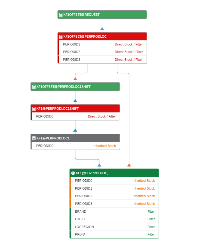
You can see that lter blocks are imposed on the following time attributes: PERIODID0, PERIODID1,
PERIODID2, and PERIODID3 throughout almost the complete calculation graph. Filtering for PERIODID0
is directly blocked because of the time attribute transformation. Additionally, it entails an inherited lter
block on this attribute in all the calculations below the attribute transformation. Filtering for PERIODID1,
PERIODID2, and PERIODID3 is directly blocked because of the inner join that returns these attributes after
the transformation. Again, lter blocks are applied on these attributes in all the calculations that are below
in the graph.
Since there are several direct and inherited lter blocks in this calculation graph, you can only lter for time
attributes at a later step of the calculation processing (after the time attribute transformation). This means
that you can only reduce data volume almost at the very end of the calculation chain, that is, the query of
KF1OFFSET will probably take a lot of time.
Model Conguration Guide
Monitoring and Troubleshooting
PUBLIC 487
4. To improve performance and speed up your query, follow the recommendations below:
• Use those attributes for ltering that can already be used for ltering at the level of the stored key
gure.
To nd ecient lter attributes, select the Only Filter Attributes option from the dropdown. Look for
attributes that can be used for ltering at the level of the stored key gure.
For example, if planners are responsible for certain products or locations only, they can use the PRDID
or LOCID attribute for ltering. This is a very eective way of ltering, since it reduces data volume
right from the beginning of the calculation chain. Calculations will be performed on a smaller set of
data and most probably will result in performance improvements.
• Consider simplifying the calculations below the time attribute transformation. This way you can avoid
peforming complex calculations on large data volumes and you can ensure that unltered data is
processed as quickly as possible.
• Separate those key gures into dierent planning view templates (in SAP IBP, add-in for Microsoft
Excel) that cannot be ltered, and thus queried eectively together.
While ltering for an attribute might prove to be eective for several key gures, it might result in lter
blocks in case of other key gures. For example, a master data attribute can act as an eective lter in
case of key gures that have time attribute transformation in their calculation graphs. However, in case
of key gures that have master data transformation in their calculation graphs, there might be lter
blocks on the very same master data attribute. Seperate these key gures into dierent planning view
templates, or make these key gures independent from each other by duplicating the commonly used
calculations.
29.4.2Example: Master Data Attribute Transformation
In this example, the calculation of the ACTUALSQTY key gure takes a lot of time, Microsoft Excel templates
are loading very slowly. To investigate what the problem might be, let's call up the Key Figure Calculations
app and search for the ACTUALSQTY key gure. By checking the calculation graph of the key gure, we learn
that the graph contains a master data transformation, which imposes lter blocks and probably causes the
performance issues. To analyze and x this problem, follow the steps below.
1. Open the Key Figure Calculations app, select your planning area and key gure (ACTUALSQTY in this case),
and then choose Go.
The calculation graph of the key gure is loaded.
2. Choose the Calculations tab rst to get an overview of the calculations in the graph.
488
PUBLIC
Model Conguration Guide
Monitoring and Troubleshooting

Here, you can see that there is a master data transformation: LOCID@MTHPRODLOCSHIFT =
"LOCFR". The LOCID master data will have the value of the LOCFR master data. To ensure the
consistency of this calculation, all the other location attributes are dropped with the aggregation
ACTUALSQTY@MTHPRODLOCSHIFT1 = SUM("ACTUALSQTY@MTHPRODLOC") and removed from the
planning level. After the transformation, they are returned with an inner join.
3. Now, choose the Filter Blocks tab and select the Show All Attributes option from the dropdown.
Model Conguration Guide
Monitoring and Troubleshooting
PUBLIC 489

You can see that lter blocks are imposed on the following location attributes: LOCID, ATDREGION,
LOCTYPE, and REGION throughout almost the complete calculation graph. Filtering for LOCID is directly
blocked because of the attribute transformation. Additionally, it entails an inherited lter block on this
attribute in all the calculations below the attribute transformation. Filtering for ATDREGION, LOCTYPE, and
REGION is directly blocked because of the inner join that returns these attributes after the transformation.
Again, lter blocks are applied on these attributes in all the calculations that are below in the graph.
Since there are several direct and inherited lter blocks in this calculation graph, you can only lter
for location attributes at a later step of the calculation processing (after the master data attribute
transformation). This means that ltering for location attributes can only reduce data volume almost at the
very end of the calculation chain, that is, the query of ACTUALSQTY will probably take a lot of time.
490
PUBLIC
Model Conguration Guide
Monitoring and Troubleshooting
4. To improve performance and speed up your query, follow the recommendations below:
• Use those attributes for ltering that can already be used for ltering at the level of the stored key
gure.
To nd ecient lter attributes, select the Only Filter Attributes option from the dropdown. Look for
attributes that can be used for ltering at the level of the stored key gure.
For example, if planners are responsible for certain products or product families only, they can use the
product attributes (PRDFAMILY and PRDID) for ltering. This is a very eective way of ltering, since it
reduces data volume right from the beginning of the calculation chain. Calculations will be performed
on a smaller set of data and most probably will result in performance improvements.
• Before shifting a key gure, do not aggregate those attributes that will not change due to the attribute
transformation. By doing so, planners can use them for ltering right from the beginning of the
calculation chain.
For example, if planners are responsible for locations that all belong to the same region, do no
aggregate REGION. This way they can lter for the region they are responsible for and speed up the
queries.
Please note that it is always the responsibility of the modeling expert to ensure that the uploaded data
complies with the modeling requirements. That is, if planners are responsible for locations that belong
to a dierent region, the calculation will produce incorrect results.
• Consider simplifying the calculations below the master data transformation. This way you can avoid
peforming complex calculations on large data volumes and you can ensure that unltered data is
processed as quickly as possible.
• Separate those key gures into dierent planning view templates (in SAP IBP, add-in for Microsoft
Excel) that cannot be ltered, and thus queried eectively together.
While ltering for an attribute might prove to be eective for several key gures, it might result in lter
blocks in case of other key gures. For example, a time attribute can act as an eective lter in case
of key gures that have master data transformation in their calculation graphs. However, in case of key
gures that have time attribute transformation in their calculation graphs, there might be lter blocks
on the very same time attribute. Seperate these key gures into dierent planning view templates, or
make these key gures independent from each other by duplicating the commonly used calculations.
29.4.3Example: Cumulative Aggregation
In this example, the calculation of the CKF03CAGGR key gure takes a lot of time, Microsoft Excel templates are
loading very slowly. To investigate what the problem might be, let's call up the Key Figure Calculations app and
search for the CKF03CAGGR key gure. By checking the calculation graph of the key gure, we learn that the
graph contains a cross-period calculation, which imposes lter blocks and probably causes the performance
issues. To analyze and x this problem, follow the steps below.
1. Open the Key Figure Calculations app, select your planning area and key gure (CKF03CAGGR in this case),
and then choose Go.
The calculation graph of the key gure is loaded.
2. Choose the Calculations tab rst to get an overview of the calculations in the graph.
Model Conguration Guide
Monitoring and Troubleshooting
PUBLIC 491

Here, you can see that there is cumulative aggregation: CKF03CAGGR@MTHPRODLOC =
IBP_CAGGR("SKF01@MTHPRODLOC" , 'MIN' , 'FORWARD' , 'FUTURE'). This is a cross-period
calculation, where the calculation of a key gure value uses values from several time periods. Due to
the cross-period nature of this calculation, you cannot lter for the time attributes before the calculation is
performed, only after it.
3. Now, choose the Filter Blocks tab and select the Show All Attributes option from the dropdown.
492
PUBLIC
Model Conguration Guide
Monitoring and Troubleshooting
You can see that due to the cumulative aggregation lter blocks are imposed on all the time
attributes (PERIODID0, PERIODID1, and PERIODID2) throughout almost the complete calculation graph.
Additionally, inherited lter blocks are raised for these attributes in all the calculations below the
cumulative aggregation. Filter blocks are required because the calculation uses inputs from various time
periods.
Since there are several direct and inherited lter blocks in this calculation graph, you can only lter for
time attributes after the cumulative aggregation has been performed. This means that ltering for time
attributes can only reduce data volume almost at the very end of the calculation chain. That is, the query of
CKF03CAGGR will operate on a large data volume and, probably will take a lot of time.
4. To improve performance and speed up your query, follow the recommendations below:
• Use those attributes for ltering that can already be used for ltering at the level of the stored key
gure.
To nd ecient lter attributes, select the Only Filter Attributes option from the dropdown. Look for
attributes that can be used for ltering at the level of the stored key gure.
For example, if planners are responsible for certain products or locations only, they can use the PRDID
or LOCID attribute for ltering. This is a very eective way of ltering, since it reduces data volume
right from the beginning of the calculation chain. Calculations will be performed on a smaller set of
data and most probably will result in performance improvements.
• Consider simplifying the calculations below the cumulative aggregation. This way you can avoid
peforming complex calculations on large data volumes and you can ensure that unltered data is
processed as quickly as possible.
• Separate those key gures into dierent planning view templates (in SAP IBP, add-in for Microsoft
Excel) that cannot be ltered, and thus queried eectively together.
While ltering for an attribute might prove to be eective for several key gures, it might result in lter
blocks in case of other key gures. For example, a master data attribute can act as an eective lter
in case of key gures that have cross-period calculation in their calculation graphs. However, in case
of key gures that have master data transformation in their calculation graphs, there might be lter
blocks on the very same master data attribute. Seperate these key gures into dierent planning view
templates, or make these key gures independent from each other by duplicating the commonly used
calculations.
29.4.4Watch a video!
Watch a video about lter blocks and eective ltering.
Model Conguration Guide
Monitoring and Troubleshooting
PUBLIC 493

Important Disclaimers and Legal Information
Hyperlinks
Some links are classied by an icon and/or a mouseover text. These links provide additional information.
About the icons:
• Links with the icon : You are entering a Web site that is not hosted by SAP. By using such links, you agree (unless expressly stated otherwise in your
agreements with SAP) to this:
• The content of the linked-to site is not SAP documentation. You may not infer any product claims against SAP based on this information.
• SAP does not agree or disagree with the content on the linked-to site, nor does SAP warrant the availability and correctness. SAP shall not be liable for any
damages caused by the use of such content unless damages have been caused by SAP's gross negligence or willful misconduct.
• Links with the icon : You are leaving the documentation for that particular SAP product or service and are entering an SAP-hosted Web site. By using
such links, you agree that (unless expressly stated otherwise in your agreements with SAP) you may not infer any product claims against SAP based on this
information.
Videos Hosted on External Platforms
Some videos may point to third-party video hosting platforms. SAP cannot guarantee the future availability of videos stored on these platforms. Furthermore, any
advertisements or other content hosted on these platforms (for example, suggested videos or by navigating to other videos hosted on the same site), are not within
the control or responsibility of SAP.
Beta and Other Experimental Features
Experimental features are not part of the ocially delivered scope that SAP guarantees for future releases. This means that experimental features may be changed by
SAP at any time for any reason without notice. Experimental features are not for productive use. You may not demonstrate, test, examine, evaluate or otherwise use
the experimental features in a live operating environment or with data that has not been suciently backed up.
The purpose of experimental features is to get feedback early on, allowing customers and partners to inuence the future product accordingly. By providing your
feedback (e.g. in the SAP Community), you accept that intellectual property rights of the contributions or derivative works shall remain the exclusive property of SAP.
Example Code
Any software coding and/or code snippets are examples. They are not for productive use. The example code is only intended to better explain and visualize the syntax
and phrasing rules. SAP does not warrant the correctness and completeness of the example code. SAP shall not be liable for errors or damages caused by the use of
example code unless damages have been caused by SAP's gross negligence or willful misconduct.
Bias-Free Language
SAP supports a culture of diversity and inclusion. Whenever possible, we use unbiased language in our documentation to refer to people of all cultures, ethnicities,
genders, and abilities.
494
PUBLIC
Model Conguration Guide
Important Disclaimers and Legal Information
Model Conguration Guide
Important Disclaimers and Legal Information
PUBLIC 495

www.sap.com/contactsap
© 2023 SAP SE or an SAP aliate company. All rights reserved.
No part of this publication may be reproduced or transmitted in any form
or for any purpose without the express permission of SAP SE or an SAP
aliate company. The information contained herein may be changed
without prior notice.
Some software products marketed by SAP SE and its distributors
contain proprietary software components of other software vendors.
National product specications may vary.
These materials are provided by SAP SE or an SAP aliate company for
informational purposes only, without representation or warranty of any
kind, and SAP or its aliated companies shall not be liable for errors or
omissions with respect to the materials. The only warranties for SAP or
SAP aliate company products and services are those that are set forth
in the express warranty statements accompanying such products and
services, if any. Nothing herein should be construed as constituting an
additional warranty.
SAP and other SAP products and services mentioned herein as well as
their respective logos are trademarks or registered trademarks of SAP
SE (or an SAP aliate company) in Germany and other countries. All
other product and service names mentioned are the trademarks of their
respective companies.
Please see https://www.sap.com/about/legal/trademark.html for
additional trademark information and notices.
THE BEST RUN
