
Dynamo Training School, Lisbon Introduction to Dynamic Networks
1
Introduction to Dynamic Networks
Models, Algorithms, and Analysis
Rajmohan Rajaraman, Northeastern U.
www.ccs.neu.edu/home/rraj/Talks/DynamicNetworks/DYNAMO/
June 2006

Dynamo Training School, Lisbon Introduction to Dynamic Networks
2
Many Thanks to…
• Filipe Araujo, Pierre Fraigniaud, Luis Rodrigues,
Roger Wattenhofer, and organizers of the summer
school
• All the researchers whose contributions will be
discussed in this tutorial

Dynamo Training School, Lisbon Introduction to Dynamic Networks
3
What is a Network?
General undirected or directed graph

Dynamo Training School, Lisbon Introduction to Dynamic Networks
4
Classification of Networks
• Synchronous:
– Messages delivered
within one time unit
– Nodes have access to a
common clock
• Asynchronous:
– Message delays are
arbitrary
– No common clock
• Static:
– Nodes never crash
– Edges maintain
operational status forever
• Dynamic:
– Nodes may come and go
– Edges may crash and
recover

Dynamo Training School, Lisbon Introduction to Dynamic Networks
5
Dynamic Networks: What?
• Network dynamics:
– The network topology changes over times
– Nodes and/or edges may come and go
– Captures faults and reliability issues
• Input dynamics:
– Load on network changes over time
– Packets to be routed come and go
– Objects in an application are added and deleted

Dynamo Training School, Lisbon Introduction to Dynamic Networks
6
Dynamic Networks: How?
• Duration:
– Transient: The dynamics occur for a short
period, after which the system is static for an
extended time period
– Continuous: Changes are constantly occurring
and the system has to constantly adapt to
them
• Control:
– Adversarial
– Stochastic
– Game-theoretic

Dynamo Training School, Lisbon Introduction to Dynamic Networks
7
Dynamic Networks are Everywhere
• Internet
– The network, traffic, applications are all
dynamically changing
• Local-area networks
– Users, and hence traffic, are dynamic
• Mobile ad hoc wireless networks
– Moving nodes
– Changing environmental conditions
• Communication networks, social networks,
Web, transportation networks, other
infrastructure

Dynamo Training School, Lisbon Introduction to Dynamic Networks
8
Adversarial Models
• Dynamics are controlled by an adversary
– Adversary decides when and where changes
occur
– Edge crashes and recoveries, node arrivals and
departures
– Packet arrival rates, sources, and destinations
• For meaningful analysis, need to constrain
adversary
– Maintain some level of connectivity
– Keep packet arrivals below a certain rate

Dynamo Training School, Lisbon Introduction to Dynamic Networks
9
Stochastic Models
• Dynamics are described by a probabilistic
process
– Neighbors of new nodes randomly selected
– Edge failure/recovery events drawn from some
probability distribution
– Packet arrivals and lengths drawn from some
probability distribution
• Process parameters are constrained
– Mean rate of packet arrivals and service time
distribution moments
– Maintain some level of connectivity in network

Dynamo Training School, Lisbon Introduction to Dynamic Networks
10
Game-Theoretic Models
• Implicit assumptions in previous two
models:
– All network nodes are under one administration
– Dynamics through external influence
• Here, each node is a potentially
independent agent
– Own utility function, and rationally behaved
– Responds to actions of other agents
– Dynamics through their interactions
• Notion of stability:
– Nash equilibrium

Dynamo Training School, Lisbon Introduction to Dynamic Networks
11
Design & Analysis Considerations
• Distributed computing:
– For static networks, can do pre-processing
– For dynamic networks (even with transient dynamics),
need distributed algorithms
• Stability:
– Transient dynamics: Self-stabilization
– Continuous dynamics: Resources bounded at all times
– Game-theoretic: Nash equilibrium
• Convergence time
• Properties of stable states:
– How much resource is consumed?
– How well is the network connected?
– How far is equilibrium from socially optimal?

Dynamo Training School, Lisbon Introduction to Dynamic Networks
12
Five Illustrative Problem Domains
• Spanning trees
– Transient dynamics, self-stabilization
• Load balancing
– Continuous dynamics, adversarial input
• Packet routing
– Transient & continuous dynamics, adversarial
• Queuing systems
– Adversarial input
• Network evolution
– Stochastic & game-theoretic

Dynamo Training School, Lisbon Introduction to Dynamic Networks
13
Spanning Trees

Dynamo Training School, Lisbon Introduction to Dynamic Networks
14
Spanning Trees
• One of the most fundamental network structures
• Often the basis for several distributed system
operations including leader election, clustering,
routing, and multicast
• Variants: any tree, BFS, DFS, minimum spanning
trees

Dynamo Training School, Lisbon Introduction to Dynamic Networks
15
Spanning Tree in a Static Network
• Assumption: Every node has a unique identifier
• The largest id node will become the root
• Each node v maintains distance d(v) and next-hop h(v) to
largest id node r(v) it is aware of:
– Node v propagates (d(v),r(v)) to neighbors
– If message (d,r) from u with r > r(v), then store (d+1,r,u)
– If message (d,r) from p(v), then store (d+1,r,p(v))
8
3
2
4
5
6
7
1

Dynamo Training School, Lisbon Introduction to Dynamic Networks
16
Spanning Tree in a Dynamic Network
• Suppose node 8 crashes
• Nodes 2, 4, and 5 detect the crash
• Each separately discards its own triple, but believes it can
reach 8 through one of the other two nodes
– Can result in an infinite loop
• How do we design a self-stabilizing algorithm?
8
3
2
4
5
6
7
1

Dynamo Training School, Lisbon Introduction to Dynamic Networks
17
Exercise
• Consider the following spanning tree algorithm in
a synchronous network
• Each node v maintains distance d(v) and next-
hop h(v) to largest id node r(v) it is aware of
• In each step, node v propagates (d(v),r(v)) to
neighbors
• On receipt of a message:
– If message (d,r) from u with r > r(v), then store
(d+1,r,u)
– If message (d,r) from p(v), then store (d+1,r,p(v))
• Show that there exists a scenario in which a node
fails, after which the algorithm never stabilizes

Dynamo Training School, Lisbon Introduction to Dynamic Networks
18
Self-Stabilization
• Introduced by Dijkstra [Dij74]
– Motivated by fault-tolerance issues [Sch93]
– Hundreds of studies since early 90s
• A system S is self-stabilizing with respect to
predicate P
– Once P is established, P remains true under no dynamics
– From an arbitrary state, S reaches a state satisfying P
within finite number of steps
• Applies to transient dynamics
• Super-stabilization notion introduced for
continuous dynamics [DH97]

Dynamo Training School, Lisbon Introduction to Dynamic Networks
19
Self-Stabilizing ST Algorithms
• Dozens of self-stabilizing algorithms for finding
spanning trees under various models [Gär03]
– Uniform vs non-uniform networks
– Fixed root vs non-fixed root
– Known bound on the number of nodes
– Network remains connected
• Basic idea:
– Some variant of distance vector approach to build a BFS
– Symmetry-breaking
• Use distinguished root or distinct ids
– Cycle-breaking
• Use known upper bound on number of nodes
• Local detection paradigm

Dynamo Training School, Lisbon Introduction to Dynamic Networks
20
Self-Stabilizing Spanning Tree
• Suppose upper bound N known on number of nodes [AG90]
• Each node v maintains distance d(v) and parent h(v) to
largest id node r(v) it is aware of:
– Node v propagates (d(v),r(v)) to neighbors
– If message (d,r) from u with r > r(v), then store (d+1,r,u)
– If message (d,r) from p(v), then store (d+1,r,p(v))
• If d(v) exceeds N, then store (0,v,v): breaks cycles
8
3
2
4
5
6
7
1

Dynamo Training School, Lisbon Introduction to Dynamic Networks
21
Self-Stabilizing Spanning Tree
• Suppose upper bound N not known [AKY90]
• Maintain triple (d(v),r(v),p(v)) as before
– If v > r(u) of all of its neighbors, then store
(0,v,v)
– If message (d,r) received from u with r > r(v),
then v “joins” this tree
• Sends a join request to the root r
• On receiving a grant, v stores (d+1,r,u)
– Other local consistency checks to ensure that
cycles and fake root identifiers are eventually
detected and removed

Dynamo Training School, Lisbon Introduction to Dynamic Networks
22
Spanning Trees: Summary
• Model:
– Transient adversarial network dynamics
• Algorithmic techniques:
– Symmetry-breaking through ids and/or a distinguished
root
– Cycle-breaking through sequence numbers or local
detection
• Analysis techniques:
– Self-stabilization paradigm
• Other network structures:
– Hierarchical clustering
– Spanners (related to metric embeddings)

Dynamo Training School, Lisbon Introduction to Dynamic Networks
23
Load Balancing
Dynamo Training School, Lisbon Introduction to Dynamic Networks
24
Load Balancing
• Each node v has w(v) tokens
• Goal: To balance the tokens among the nodes
• Imbalance: max
u,v
|w(u) - w
avg
|
• In each step, each node can send at most one
token to each of its neighbors

Dynamo Training School, Lisbon Introduction to Dynamic Networks
25
Load Balancing
• In a truly balanced configuration, we have |w(u) - w(v)| ≤ 1
• Our goal is to achieve fast approximate balancing
• Preprocessing step in a parallel computation
• Related to routing and counting networks [PU89, AHS91]

Dynamo Training School, Lisbon Introduction to Dynamic Networks
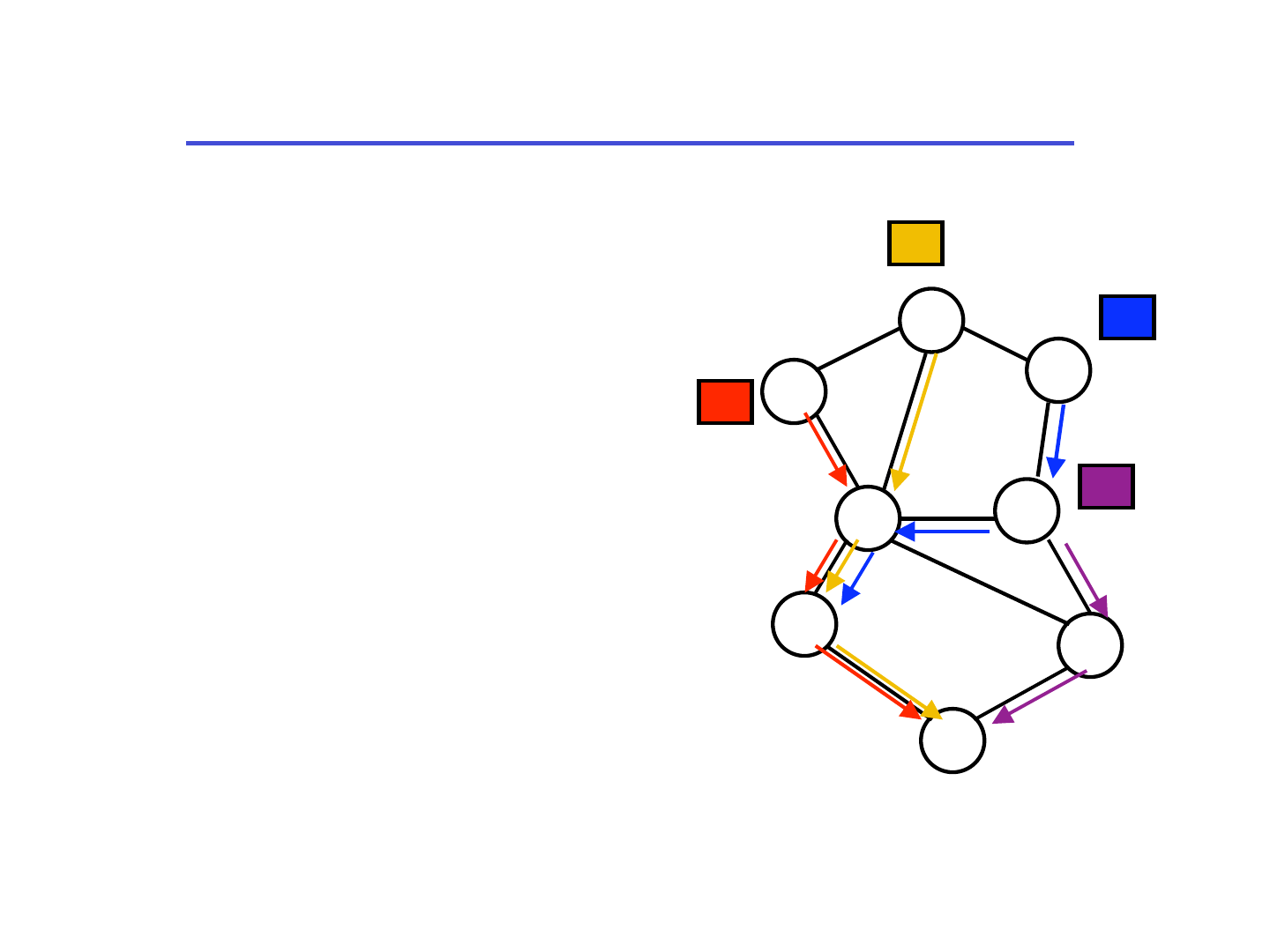
26
Local Balancing
• Each node compares its
number of tokens with its
neighbors
• In each step, for each
edge (u,v):
– If w(u) > w(v) + 2d, then u
sends a token to v
– Here, d is maximum degree
of the network
• Purely local operation

Dynamo Training School, Lisbon Introduction to Dynamic Networks
27
Convergence to Stable State
• How long does it take local balancing to
converge?
• What does it mean to converge?
– Imbalance is “constant” and remains so
• What do we mean by “how long”?
– The number of time steps it takes to achieve
the above imbalance
– Clearly depends on the topology of the network
and the imbalance of the original token
distribution

Dynamo Training School, Lisbon Introduction to Dynamic Networks
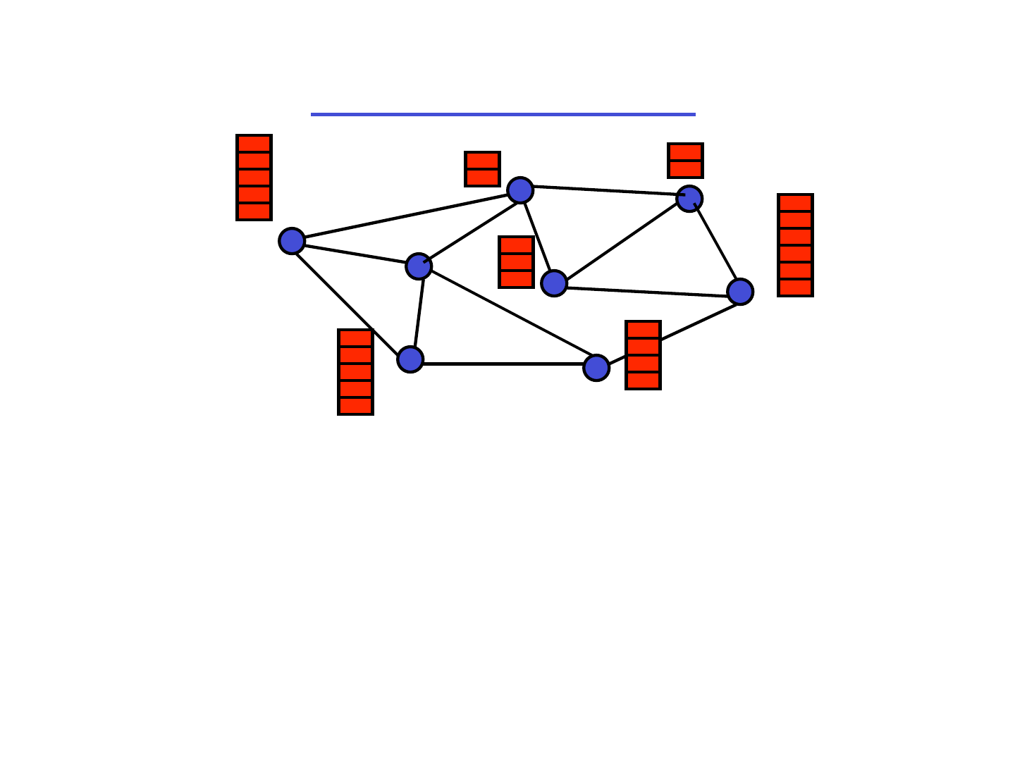
28
Expansion of a Network
• Edge expansion α:
– Minimum, over all sets S of size
≤ n/2, of the term
|E(S)|/|S|
• Lower bound on convergence
time:
(w(S) - |S|·w
avg
)/E(S)
= (w(S)/|S| - w
avg
)/ α
Expansion = 12/6 = 2
Lower bound = (29 - 18)/12
w
avg
= 3

Dynamo Training School, Lisbon Introduction to Dynamic Networks
29
Properties of Local Balancing
• For any network G with expansion α, any
token distribution with imbalance Δ converges
to a distribution with imbalance O(d·log(n)/ α)
in O(Δ/ α) steps [AAMR93, GLM+99]
• Analysis technique:
– Associate a potential with every node v, which is a
function of the w(v)
• Example: (w(v) - avg)
2
, c
w(v)-avg
• Potential of balanced configuration is small
– Argue that in every step, the potential decreases by
a desired amount (or fraction)
– Potential decrease rate yields the convergence time
• There exist distributions with imbalance Δ that
would take Ω(Δ/ α) steps

Dynamo Training School, Lisbon Introduction to Dynamic Networks
30
Exercise
• For any graph G with edge expansion α,
show that there is an initial distribution
with imbalance Δ such that the time taken
to reduce the imbalance by even half is
Ω(Δ/ α) steps

Dynamo Training School, Lisbon Introduction to Dynamic Networks
31
Local Balancing in Dynamic Networks
• The “purely local” nature of the algorithm useful
for dynamic networks
• Challenge:
– May not “know” the correct load on neighbors since
links are going up and down
• Key ideas:
– Maintain an estimate of the neighbors’ load, and
update it whenever the link is live
– Be more conservative in sending tokens
• Result:
– Essentially same as for static networks, with a slightly
higher final imbalance, under the assumption that the
the set of live edges form a network with edge
expansion α at each step

Dynamo Training School, Lisbon Introduction to Dynamic Networks
32
Adversarial Load Balancing
• Dynamic load [MR02]
– Adversary inserts and/or
deletes tokens
• In each step:
– Balancing
– Token insertion/deletion
• For any set S, let d
t
(S) be
the change in number of
tokens at step t
• Adversary is constrained in
how much imbalance can
be increased in a step
• Local balancing is stable
against rate 1 adversaries
[AKK02]
d
t
(S) – (avg
t+1
– avg
t
)|S| ≤ r · e(S)

Dynamo Training School, Lisbon Introduction to Dynamic Networks
33
Stochastic Adversarial Input
• Studied under a different model [AKU05]
– Any number of tokens can be exchanged per step, with
one neighbor
• Local balancing in this model [GM96]
– Select a random matching
– Perform balancing across the edges in matching
• Load consumed by nodes
– One token per step
• Load placed by adversary under statistical
constraints
– Expected injected load within window of w steps is at
most rnw
– The pth moment of total injected load is bounded, p > 2
• Local balancing is stable if r < 1

Dynamo Training School, Lisbon Introduction to Dynamic Networks
34
Load Balancing: Summary
• Algorithmic technique:
– Local balancing
• Design technique:
– Obtain a purely distributed solution for static
network, emphasizing local operations
– Extend it to dynamic networks by maintaining
estimates
• Analysis technique:
– Potential function method
– Martingales

Dynamo Training School, Lisbon Introduction to Dynamic Networks
35
Packet Routing

Dynamo Training School, Lisbon Introduction to Dynamic Networks
36
The Packet Routing Problem
• Given a network and a set of packets with source-
destination pairs
– Path selection: Select paths between sources and
respective destinations
– Packet forwarding: Forward the packets to the destinations
along selected paths
• Dynamics:
– Network: edges and their capacities
– Input: Packet arrival rates and locations
• Interconnection networks [Lei91], Internet [Hui95],
local-area networks, ad hoc networks [Per00]

Dynamo Training School, Lisbon Introduction to Dynamic Networks
37
Packet Routing: Performance
• Static packet set:
– Congestion of selected paths: Number of paths that
intersect at an edge/node
– Dilation: Length of longest path
• Dynamic packet set:
– Throughput: Rate at which packets can be delivered to
their destination
– Delay: Average time difference between packet release
at source and its arrival at destination
• Dynamic network:
– Communication overhead due to a topology change
– In highly dynamic networks, eventual delivery?
• Compact routing:
– Sizes of routing tables

Dynamo Training School, Lisbon Introduction to Dynamic Networks
38
Routing Algorithms Classification
• Global:
– All nodes have complete
topology information
• Decentralized:
– Nodes know information
about neighboring nodes
and links
• Static:
– Routes change rarely
over time
• Dynamic:
– Topology changes
frequently requiring
dynamic route updates
• Proactive:
– Nodes constantly react to topology changes always
maintaining routes of desired quality
• Reactive:
– Nodes select routes on demand

Dynamo Training School, Lisbon Introduction to Dynamic Networks
39
Link State Routing
• Each node periodically
broadcasts state of its links
to the network
• Each node has current state
of the network
• Computes shortest paths to
every node
– Dijkstra’s algorithm
• Stores next hop for each
destination
A
E
F
B
G
C
D
H

Dynamo Training School, Lisbon Introduction to Dynamic Networks
40
Link State Routing, contd
• When link state changes, the
broadcasts propagate
change to entire network
• Each node recomputes
shortest paths
• High communication
complexity
• Not effective for highly
dynamic networks
• Used in intra-domain routing
– OSPF
A
E
F
B
G
C
D
H

Dynamo Training School, Lisbon Introduction to Dynamic Networks
41
Distance Vector Routing
• Distributed version of
Bellman-Ford’s algorithm
• Each node maintains a
distance vector
– Exchanges with neighbors
– Maintains shortest path
distance and next hop
• Basic version not self-
stabilizing
– Use bound on number of
nodes or path length
– Poisoned reverse
G
D
H
A 5 G
B 6 G
A 4 E
B 5 E
A 3 C
B 6 G
A 4 D
B 6 G

Dynamo Training School, Lisbon Introduction to Dynamic Networks
42
Distance Vector Routing
• Basis for two routing
protocols for mobile ad
hoc wireless networks
• DSDV: proactive,
attempts to maintain
routes
• AODV: reactive, computes
routes on-demand using
distance vectors [PBR99]
G
D
H
A 4 E
B 5 E
A 3 C
B 6 G
A 4 D
B 6 G

Dynamo Training School, Lisbon Introduction to Dynamic Networks
43
Link Reversal Routing
• Aimed at dynamic networks in
which finding a single path is a
challenge [GB81]
• Focus on a destination D
• Idea: Impose direction on links
so that all paths lead to D
• Each node has a height
– Height of D = 0
– Links are directed from high to
low
• D is a sink
• By definition, we have a
directed cyclic graph
A
E
F
B
G
C
D
H
0
1
3
5
4
5
4
2
0
3
1
5
4
5
4
2

Dynamo Training School, Lisbon Introduction to Dynamic Networks
44
Setting Node Heights
• If destination D is the only
sink, then all directed
paths lead to D
• If another node is a sink,
then it reverses all links:
– Set its height to 1 more than
the max neighbor height
• Repeat until D is only sink
• A potential function
argument shows that this
procedure is self-
stabilizing
A
E
F
B
G
C
D
H
0
3
1
5
4
5
4
2
6
7

Dynamo Training School, Lisbon Introduction to Dynamic Networks
45
Exercise
• For tree networks, show that the link
reversal algorithm self-stabilizes from an
arbitrary state

Dynamo Training School, Lisbon Introduction to Dynamic Networks
46
Issues with Link Reversal
• A local disruption could cause global change in
the network
– The scheme we studied is referred to as full link
reversal
– Partial link reversal
• When the network is partitioned, the
component without sink has continual
reversals
– Proposed protocol for ad hoc networks (TORA)
attempts to avoid these [PC97]
• Need to maintain orientations of each edge for
each destination
• Proactive: May incur significant overhead for
highly dynamic networks

Dynamo Training School, Lisbon Introduction to Dynamic Networks
47
Routing in Highly Dynamic Networks
• Highly dynamic network:
– The network may not even
be connected at any point
of time
• Problem: Want to route a
message from source to
sink with small overhead
• Challenges:
– Cannot maintain any paths
– May not even be able to
find paths on demand
– May still be possible to
route!
A
E
F
B
G
C
D
H

Dynamo Training School, Lisbon Introduction to Dynamic Networks
48
End-to-End Communication
• Consider basic case of one source-destination pair
• Need redundancy since packet sent in wrong
direction may get stuck in disconnected portion!
• Slide protocol (local balancing) [AMS89, AGR92]
– Each node has an ordered queue of at most n slots for
each incoming link (same for source)
– Packet moved from slot i at node v to slot j at the (v,u)-
queue of node u only if j < i
– All packets absorbed at destination
– Total number of packets in system at most C = O(nm)

Dynamo Training School, Lisbon Introduction to Dynamic Networks
49
End-to-End Communication
• End-to-end communication using slide
• For each data item:
– Sender sends 2C+1 copies of item (new token added only if
queue is not full)
– Receiver waits for 2C+1 copies and outputs majority
• Safety: The receiver output is always prefix of sender input
• Liveness: If the sender and the receiver are eventually
connected:
– The sender will eventially input a new data item
– The receiver eventually outputs the data item
• Strong guarantees considering weak connectivity
• Overhead can be reduced using coding e.g. [Rab89]

Dynamo Training School, Lisbon Introduction to Dynamic Networks
50
Routing Through Local Balancing
• Multi-commodity flow [AL94]
• Queue for each flow’s packets at
head and tail of each edge
• In each step:
– New packets arrive at sources
– Packet(s) transmitted along each
edge using local balancing
– Packets absorbed at destinations
– Queues balanced at each node
• Local balancing through potentials
– Packets sent along edge to maximize
potential drop, subject to capacity
• Queues balanced at each node by
simply distributing packets evenly
ϕ
k
(q) = exp(εq/(8Ld
k
)
L = longest path length
d
k
= demand for flow k

Dynamo Training School, Lisbon Introduction to Dynamic Networks
51
Routing Through Local Balancing
• Edge capacities can be dynamically
and adversarially changing
• If there exists a feasible flow that
can route d
k
flow for all k:
– This routing algorithm will route (1-
eps) d
k
for all k
• Crux of the argument:
– Destination is a sink and the source
is constantly injecting new flow
– Gradient in the direction of the sink
– As long as feasible flow paths exist,
there are paths with potential drop
• Follow-up work has looked at packet
delays and multicast problems
[ABBS01, JRS03]
ϕ
k
(q) = exp(εq/(8Ld
k
)
L = longest path length
d
k
= demand for flow k

Dynamo Training School, Lisbon Introduction to Dynamic Networks
52
Packet Routing: Summary
• Models:
– Transient and continuous dynamics
– Adversarial
• Algorithmic techniques:
– Distance vector
– Link reversal
– Local balancing
• Analysis techniques:
– Potential function

Dynamo Training School, Lisbon Introduction to Dynamic Networks
53
Queuing Systems

Dynamo Training School, Lisbon Introduction to Dynamic Networks
54
Packet Routing: Queuing
• We now consider the
second aspect of routing:
queuing
• Edges have finite capacity
• When multiple packets
need to use an edge, they
get queued in a buffer
• Packets forwarded or
dropped according to
some order
A
E
F
B
G
C
D
H
D
D
D
D
D
D
D
D

Dynamo Training School, Lisbon Introduction to Dynamic Networks
55
Packet Queuing Problems
• In what order should the packets be forwarded?
– First in first out (FIFO or FCFS)
– Farthest to go (FTG), nearest to go (NTG)
– Longest in system (LIS), shortest in system (SIS)
• Which packets to drop?
– Tail drop
– Random early detection (RED)
• Major considerations:
– Buffer sizes
– Packet delays
– Throughput
• Our focus: forwarding

Dynamo Training School, Lisbon Introduction to Dynamic Networks
56
Dynamic Packet Arrival
• Dynamic packet arrivals in static networks
– Packet arrivals: when, where, and how?
– Service times: how long to process?
• Stochastic model:
– Packet arrival is a stochastic process
– Probability distribution on service time
– Sources, destinations, and paths implicitly constrained by
certain load conditions
• Adversarial model:
– Deterministic: Adversary decides packet arrivals,
sources, destinations, paths, subject to deterministic
load constraints
– Stochastic: Load constraints are stochastic

Dynamo Training School, Lisbon Introduction to Dynamic Networks
57
(Stochastic) Queuing Theory
• Rich history [Wal88, Ber92]
– Single queue, multiple parallel queues very well-
understood
• Networks of queues
– Hard to analyze owing to dependencies that arise
downstream, even for independent packet arrivals
– Kleinrock independence assumption
– Fluid model abstractions
• Multiclass queuing networks:
– Multiple classes of packets
– Packet arrivals by time-invariant independent processes
– Service times within a class are indistinguishable
– Possible priorities among classes

Dynamo Training School, Lisbon Introduction to Dynamic Networks
58
Load Conditions & Stability
• Stability:
– Finite upper bound on queues & delays
• Load constraint:
– The rate at which packets need to traverse an edge
should not exceed its capacity
• Load conditions are not sufficient to guarantee
stability of a greedy queuing policy [LK91, RS92]
– FIFO can be unstable for arbitrarily small load [Bra94]
– Different service distributions for different classes
• For independent and time-invariant packet arrival
distributions, with class-independent service
times [DM95, RS92, Bra96]
– FIFO is stable as long as basic load constraint holds
Dynamo Training School, Lisbon Introduction to Dynamic Networks
59
Adversarial Queuing Theory
• Directed network
• Packets, released at source,
travel along specified paths,
absorbed at destination
• In each step, at most one
packet sent along each edge
• Adversary injects requests:
– A request is a packet and a
specified path
• Queuing policy decides which
packet sent at each step along
each edge
• [BKR+96, BKR+01]
A
E
F
B
G
C
D
H

Dynamo Training School, Lisbon Introduction to Dynamic Networks
60
Load Constraints
• Let N(T,e) be number of paths
injected during interval T that
traverse e
• (w,r)-adversary:
– For any interval T of w consecutive
time steps, for every edge e:
N(T,e) ≤ w · r
– Rate of adversary is r
• (w,r) stochastic adversary:
– For any interval [t+1…t+w], for
every edge e:
E[N(T,e)|H
t
] ≤ w · r
t
# paths using e
injected at t
w
Area ≤ w · r
e

Dynamo Training School, Lisbon Introduction to Dynamic Networks
61
Stability in DAGs
• Theorem: For any dag, any greedy
policy is stable against any rate-1
adversary
• A
t
(e) = # packets in network at
time t that will eventually use e
• Q
t
(e) = queue size for e at time t
• Proof: time-invariant upper bound
on A
t
(e)
Large queue: Q
t-w
(e) ≥ w ⇒ A
t
(e) ≤ A
t-w
(e)
Small queue: Q
t-w
(e) < w ⇒ A
t-w
(e) ≤ w + ∑
j
A
t-w
(e
j
)
A
t
(e) ≤ 2w + ∑
j
A
t-w
(e
j
)
e
e
1
e
2
e
3

Dynamo Training School, Lisbon Introduction to Dynamic Networks
62
Extension to Stochastic Adversaries
• Theorem: In DAGs, any greedy policy is stable
against any stochastic 1-ε rate adversary, for any
ε>0
• Cannot claim a hard upper bound on A
t
(e)
• Define a potential ϕ
t
, that is an upper bound on
the number of packets in system
• Show that if the potential is larger than a
specified constant, then there is an expected
decrease in the next step
• Invoke results from martingale theory to argue
that E[ϕ
t
] is bounded by a constant

Dynamo Training School, Lisbon Introduction to Dynamic Networks
63
FIFO is Unstable [A+ 96]
• Initially: s packets waiting
at A to go to C
• Next s steps:
– rs packets for loop
– rs packets for B-C
• Next rs steps:
– r
2
s packets from B to A
– r
2
s packets for B-C
• Next r
2
s steps:
– r
3
s packets for C-A
• Now: s+1 packets waiting
at C going to A
• FIFO does not use edges
most effectively
A
B
C
D

Dynamo Training School, Lisbon Introduction to Dynamic Networks
64
Stability in General Networks
• LIS and SIS are universally stable against rate <1
adversaries [AAF+96]
• Furthest-To-Go and Nearest-To-Origin are stable
even against rate 1 adversaries [Gam99]
• Bounds on queue size:
– Mostly exponential in the length of the shortest path
– For DAGs, Longest-In-System (LIS) has poly-sized
queues
• Bounds on packet delays:
– A variant of LIS has poly-sized packet delays

Dynamo Training School, Lisbon Introduction to Dynamic Networks
65
Exercise
• Are the following two equivalent? Is one
stronger than the other?
– A finite bound on queue sizes
– A finite bound on delay of each packet

Dynamo Training School, Lisbon Introduction to Dynamic Networks
66
Queuing Theory: Summary
• Focus on input dynamics in static networks
• Both stochastic and adversarial models
• Primary concern: stability
– Finite bound on queue sizes
– Finite bound on packet delays
• Algorithmic techniques: simple greedy policies
• Analysis techniques:
– Potential functions
– Markov chains and Markov decision processes
– Martingales

Dynamo Training School, Lisbon Introduction to Dynamic Networks
67
Network Evolution

Dynamo Training School, Lisbon Introduction to Dynamic Networks
68
How do Networks Evolve?
• Internet
– New random graph models
– Developed to support observed properties
• Peer-to-peer networks
– Specific structures for connectivity properties
– Chord [SMK+01], CAN [RFH+01], Oceanstore
[KBC+00], D2B [FG03], [PRU01], [LNBK02], …
• Ad hoc networks
– Connectivity & capacity [GK00…]
– Mobility models [BMJ+98, YLN03, LNR04]

Dynamo Training School, Lisbon Introduction to Dynamic Networks
69
Internet Graph Models
• Internet measurements [FFF99, TGJ+02,
…]:
– Degrees follow heavy-tailed distribution at the
AS and router levels
– Frequency of nodes with degree d is
proportional to 1/d
β
, 2 < β < 3
• Models motivated by these observations
– Preferential attachment model [BA99]
– Power law graph model [ACL00]
– Bicriteria optimization model [FKP02]

Dynamo Training School, Lisbon Introduction to Dynamic Networks
70
Preferential Attachment
• Evolutionary model [BA99]
• Initial graph is a clique of size
d+1
– d is degree-related parameter
• In step t, a new node arrives
• New node selects d neighbors
• Probability that node j is
neighbor is proportional to its
current degree
• Achieves power law degree
distribution

Dynamo Training School, Lisbon Introduction to Dynamic Networks
71
Power Law Random Graphs
• Structural model [ACL00]
• Generate a graph with a specified degree
sequence (d
1
,…,d
n
)
– Sampled from a power law degree distribution
• Construct d
j
mini-vertices for each j
• Construct a random perfect matching
• Graph obtained by adding an edge for every edge
between mini-vertices
• Adapting for Internet:
– Prune 1- and 2-degree vertices repeatedly
– Reattach them using random matchings

Dynamo Training School, Lisbon Introduction to Dynamic Networks
72
Bicriteria Optimization
• Evolutionary model
• Tree generation with power law
degrees [FKP02]
• All nodes in unit square
• When node j arrives, it attaches
to node k that minimizes:
α · d
jk
+ h
k
• If 4 ≤ α ≤ o(√n):
– Degrees distributed as power
law for some β, dependent on α
• Can be generalized, but no
provable results known
h
k
: measure of centrality
of k in tree

Dynamo Training School, Lisbon Introduction to Dynamic Networks
73
Connectivity & Capacity Properties
• Congestion in certain uniform multicommodity flow
problems:
– Suppose each pair of nodes is a source-destination pair for a
unit flow
– What will be the congestion on the most congested edge of
the graph, assuming uniform capacities
– Comparison with expander graphs, which would tend to have
the least congestion
• For power law graphs with constant average degree,
congestion is O(n log
2
n) with high probability [GMS03]
– Ω(n) is a lower bound
• For preferential attachment model, congestion is O(n log n)
with high probability [MPS03]
• Analysis by proving a lower bound on conductance, and
hence expansion of the network

Dynamo Training School, Lisbon Introduction to Dynamic Networks
74
Network Creation Game
• View Internet as the product
of the interaction of many
economic agents
• Agents are nodes and their
strategy choices create the
network
• Strategy s
j
of node j:
– Edges to a subset of the nodes
• Cost c
j
for node j:
– α·|s
j
| + ∑
k
d
G(s)
(j,k)
– Hardware cost plus quality of
service costs
3α + sum of distances to
all nodes

Dynamo Training School, Lisbon Introduction to Dynamic Networks
75
Network Creation Game
• In the game, each node selects the
best response to other nodes’
strategies
• Nash equilibrium s:
– For all j, c
j
(s) ≤ c
j
(s’) for all s’ that
differ from s only in the jth
component
• Price of anarchy [KP99]:
– Maximum, over all Nash equilibria, of
the ratio of total cost in equilibrium to
smallest total cost
• Bound, as a function of α [AEED06]:
– O(1) for α = O(√n) or Ω(n log n)
– Worst-case ratio O(n
1/3
)

Dynamo Training School, Lisbon Introduction to Dynamic Networks
76
Other Network Games
• Variants of network creation games
– Weighted version [AEED06]
– Cost and benefit tradeoff [BG00]
• Cost sharing in network design [JV01,
ADK04, GST04]
• Congestion games [RT00, Rou02]
– Each source-destination pair selects a path
– Delay on edge is a function of the number of
flows that use the edge

Dynamo Training School, Lisbon Introduction to Dynamic Networks
77
Network Evolution: Summary
• Models:
– Stochastic
– Game-theoretic
• Analysis techniques:
– Graph properties, e.g., expansion, conductance
– Probabilistic techniques
– Techniques borrowed from random graphs
